

1. Start Snowflake query optimization with a measurable question
Snowflake query optimization is the process of identifying a query bottleneck, changing the relevant SQL or compute setting and verifying both results and measured behavior. Start with Query Profile and a clear report grain. A shorter query or a larger warehouse does not automatically make the workload better.
In this original lab, a retailer needs January sales by customer region. You will generate 100,000 synthetic order rows, establish dimension uniqueness, compare two valid query shapes, preserve query IDs and reconcile identical outputs. The expected January result is 31,000 orders and total amount 166,000.00. Performance numbers must come from your own account.
This is an intermediate SQL guide. It complements the Snowflake architecture guide, while keeping its focus on diagnosis and a repeatable experiment. It does not replace the separate Dynamic Tables tutorial or CDC workflow.
Reference: Exploring query execution times.
2. Classify the delay before changing SQL
| Evidence | Likely investigation | First experiment |
|---|---|---|
| High compilation time | SQL generation, complex plan or object expansion | Simplify only after reviewing the actual plan |
| High queued overload time | Concurrent demand exceeds available execution capacity | Review workload scheduling or concurrency configuration |
| Large TableScan share | Columns, filters and micro-partition pruning | Compare selected columns and scan/partition statistics |
| Join output unexpectedly larger than input | Missing join condition or nonunique business keys | Check grain and duplicate keys before tuning |
| Local or remote spill | Intermediate data exceeds available memory | Reduce rows/columns or evaluate suitable warehouse capacity |
| Repeated query returns very quickly | Result reuse or warm warehouse data | Separate cache behavior from execution work |
These are investigation directions, not automatic diagnoses. A slow scan can be appropriate for a report that legitimately needs most of a table. A large join can be correct for a many-to-many analysis. Connect each metric to the actual business requirement.
3. Set up a small, isolated and bounded lab
Use an approved database and an existing small practice warehouse. This lab needs schema/table creation, SELECT and access to your own query history. Administrative performance features and another user’s query profiles may require additional permissions.
- Record the current role, warehouse size, session parameters and whether other users share the warehouse.
- Use a fresh BA_QO_LAB schema. If it already exists, inspect the earlier exercise or select a new name; do not silently replace it.
- Start with 100,000 rows. It demonstrates validation and plan inspection, but may run too quickly to expose a meaningful performance difference.
- Keep dataset size, warehouse and business output unchanged while comparing the two SQL shapes.
- Review budget and account controls before increasing data volume or warehouse capacity. No speedup or credit saving is promised.
USE DATABASE YOUR_LAB_DATABASE;
USE WAREHOUSE YOUR_LAB_WAREHOUSE;
CREATE SCHEMA BA_QO_LAB;
USE SCHEMA BA_QO_LAB;
SELECT CURRENT_ROLE(),CURRENT_WAREHOUSE(),CURRENT_DATABASE(),CURRENT_SCHEMA();
SHOW PARAMETERS LIKE 'USE_CACHED_RESULT' IN SESSION;
SHOW PARAMETERS LIKE 'QUERY_TAG' IN SESSION;
Save the original parameter values for restoration. Warehouse compute, stored test data and optional optimization services have costs. Keep this lab’s basic SQL experiment separate from features such as automatic clustering or search optimization, which require their own justification and cost review.
4. Generate a deterministic dataset and validate the grain
CREATE TABLE DIM_CUSTOMER AS
SELECT n AS customer_id,
 CASE MOD(n,4) WHEN 0 THEN 'East' WHEN 1 THEN 'West'
 WHEN 2 THEN 'North' ELSE 'South' END AS region
FROM (SELECT ROW_NUMBER() OVER(ORDER BY SEQ4()) AS n
 FROM TABLE(GENERATOR(ROWCOUNT=>100)));

CREATE TABLE FACT_ORDER AS
SELECT n AS order_id,MOD(n,100)+1 AS customer_id,
 DATEADD('day',MOD(n,100),'2026-01-01'::TIMESTAMP_NTZ) AS order_ts,
 (MOD(n,10)+1)::NUMBER(12,2) AS amount
FROM (SELECT ROW_NUMBER() OVER(ORDER BY SEQ4()) AS n
 FROM TABLE(GENERATOR(ROWCOUNT=>100000)));

SELECT COUNT(*) AS orders,COUNT(DISTINCT order_id) AS distinct_orders
FROM FACT_ORDER;
SELECT customer_id,COUNT(*) AS copies FROM DIM_CUSTOMER
GROUP BY customer_id HAVING COUNT(*)>1;
SELECT COUNT(*) AS missing_customers FROM FACT_ORDER f
LEFT JOIN DIM_CUSTOMER c USING(customer_id) WHERE c.customer_id IS NULL;
Expect 100,000 orders, 100,000 distinct order IDs, no duplicate customer keys and zero missing customers. ROW_NUMBER creates the contiguous lab sequence; do not assume an arbitrary sequence-generating function is gap-free.
SELECT COUNT(*) AS january_orders,SUM(amount) AS january_amount
FROM FACT_ORDER
WHERE order_ts>='2026-01-01'::TIMESTAMP_NTZ
 AND order_ts<'2026-02-01'::TIMESTAMP_NTZ;
Expected: 31,000 and 166,000.00. Each of the 100 day offsets occurs 1,000 times; January covers offsets 0–30. The amounts for those offsets sum to 166 per cycle. This independent arithmetic gives a useful acceptance check before you compare queries.
5. Capture a valid baseline query and its real query ID
First inspect and save the original session values from section 3. Disable persisted result reuse only for this controlled test. This does not clear the warehouse’s local data cache or make the experiment a cold-start benchmark.
ALTER SESSION SET USE_CACHED_RESULT=FALSE;
ALTER SESSION SET QUERY_TAG='BA_QO_BASELINE';
SELECT c.region,COUNT(*) AS order_count,SUM(f.amount) AS amount
FROM FACT_ORDER f JOIN DIM_CUSTOMER c USING(customer_id)
WHERE CAST(f.order_ts AS DATE) BETWEEN '2026-01-01'::DATE AND '2026-01-31'::DATE
GROUP BY c.region ORDER BY c.region;
SET baseline_qid=LAST_QUERY_ID();
-- Save the SELECT output outside the measured SELECT itself.
CREATE TEMP TABLE BASELINE_RESULT AS
SELECT * FROM TABLE(RESULT_SCAN($baseline_qid));
Capture LAST_QUERY_ID immediately after the report SELECT in the same worksheet session. The subsequent CREATE TABLE is evidence storage, not the query whose execution you are comparing. Keep its cost and timing separate.
The cast-based filter is a valid baseline for this controlled TIMESTAMP_NTZ dataset. We do not assume it necessarily causes a full scan: Snowflake may simplify expressions. The point is to inspect what the plan actually did before declaring that the rewrite improved pruning.
Reference: Persisted result reuse and session control.
6. Read Query Profile from the captured baseline
- Open Query History in Snowsight and locate the actual baseline query ID. Confirm that the SQL text is the report SELECT.
- Separate total, compilation, queue and execution time. A query waiting for a warehouse is different from an expensive join.
- Open Query Profile. Identify the most expensive operator and follow the flow of rows through scan, join, aggregate and sort.
- At TableScan, record partitions scanned/total, bytes scanned and filters. At Join, compare input/output rows. At memory-intensive operators, inspect spill.
- Save your own screenshot with sensitive values removed. Do not copy an unrelated profile and label it as this lab.
SELECT * FROM TABLE(GET_QUERY_OPERATOR_STATS($baseline_qid));
SELECT query_id,query_tag,warehouse_size,total_elapsed_time,
 compilation_time,execution_time,queued_overload_time,
 bytes_scanned,partitions_scanned,partitions_total,
 bytes_spilled_to_local_storage,bytes_spilled_to_remote_storage
FROM TABLE(INFORMATION_SCHEMA.QUERY_HISTORY_BY_SESSION(RESULT_LIMIT=>100))
WHERE query_id=$baseline_qid;
Timing fields in query history are milliseconds; byte fields are not elapsed time. Missing profile information or a permissions error is not a zero-cost result. Operator statistics are available for supported completed queries within the documented recent window.
Reference: GET_QUERY_OPERATOR_STATS.
Reference: Information Schema query history.
7. Compare a selective range and pre-aggregation query
The alternative expresses January as a half-open timestamp range and aggregates orders to customer grain before joining the unique customer table. It must preserve the report’s region-level count and amount. The schema check in section 4 is a precondition: joining a duplicated dimension changes the meaning.
ALTER SESSION SET QUERY_TAG='BA_QO_CANDIDATE';
WITH customer_month AS (
 SELECT customer_id,COUNT(*) AS order_count,SUM(amount) AS amount
 FROM FACT_ORDER
 WHERE order_ts>='2026-01-01'::TIMESTAMP_NTZ
  AND order_ts<'2026-02-01'::TIMESTAMP_NTZ
 GROUP BY customer_id
)
SELECT c.region,SUM(m.order_count) AS order_count,SUM(m.amount) AS amount
FROM customer_month m JOIN DIM_CUSTOMER c USING(customer_id)
GROUP BY c.region ORDER BY c.region;
SET candidate_qid=LAST_QUERY_ID();
CREATE TEMP TABLE CANDIDATE_RESULT AS
SELECT * FROM TABLE(RESULT_SCAN($candidate_qid));
A half-open range includes all January timestamps without inventing a last millisecond of the month. It also makes the intended boundary easy to review. A pre-aggregation can reduce rows reaching the join; it adds an aggregation step, so it is not universally faster. On this small dataset the optimizer may produce similar plans.
Review scan and join statistics for both query IDs. Keep or reject the candidate based on correct output and measured workload behavior, not SQL length or a generic rule about CTEs.
Reference: Micro-partitions and pruning.
8. Prove equivalence before comparing runtime
SELECT 'BASELINE_ONLY' AS issue,* FROM (
 SELECT * FROM BASELINE_RESULT MINUS SELECT * FROM CANDIDATE_RESULT
)
UNION ALL
SELECT 'CANDIDATE_ONLY' AS issue,* FROM (
 SELECT * FROM CANDIDATE_RESULT MINUS SELECT * FROM BASELINE_RESULT
);
SELECT 'BASELINE' AS version,SUM(order_count) AS orders,SUM(amount) AS amount
FROM BASELINE_RESULT
UNION ALL
SELECT 'CANDIDATE',SUM(order_count),SUM(amount) FROM CANDIDATE_RESULT;
The difference query should return zero rows. Both summary rows should show 31,000 orders and 166,000.00. MINUS uses set semantics, so also confirm the output key is unique:
SELECT region,COUNT(*) FROM BASELINE_RESULT GROUP BY region HAVING COUNT(*)>1;
SELECT region,COUNT(*) FROM CANDIDATE_RESULT GROUP BY region HAVING COUNT(*)>1;
Both duplicate-key checks should be empty. Count and total checks alone could conceal an amount moving between regions. The two-way difference checks each region’s values, while the uniqueness checks protect the intended output grain.
8.1 Test a changed boundary, not just the happy path
Add one disposable order at exactly 2026-02-01 00:00:00 with a large amount and rerun both January SELECTs. January totals must remain unchanged. Use a fresh order ID and restore the seed only in the isolated lab. This tests the exclusion boundary; it does not measure speed.
INSERT INTO FACT_ORDER VALUES
 (100001,1,'2026-02-01 00:00:00'::TIMESTAMP_NTZ,9999.00);
-- Rerun both January report SELECTs: still 31,000 and 166,000.00.
-- After recording the boundary test:
DELETE FROM FACT_ORDER WHERE order_id=100001;
Run the DELETE only in your disposable lab after checking that this ID belongs to the inserted test row. Record the boundary test separately from the unchanged-dataset benchmark.
9. Run a fair experiment without invented speedups
- Use the same validated dataset and warehouse configuration for both versions. Do not compare one busy shared-warehouse run against an idle run and call it a SQL improvement.
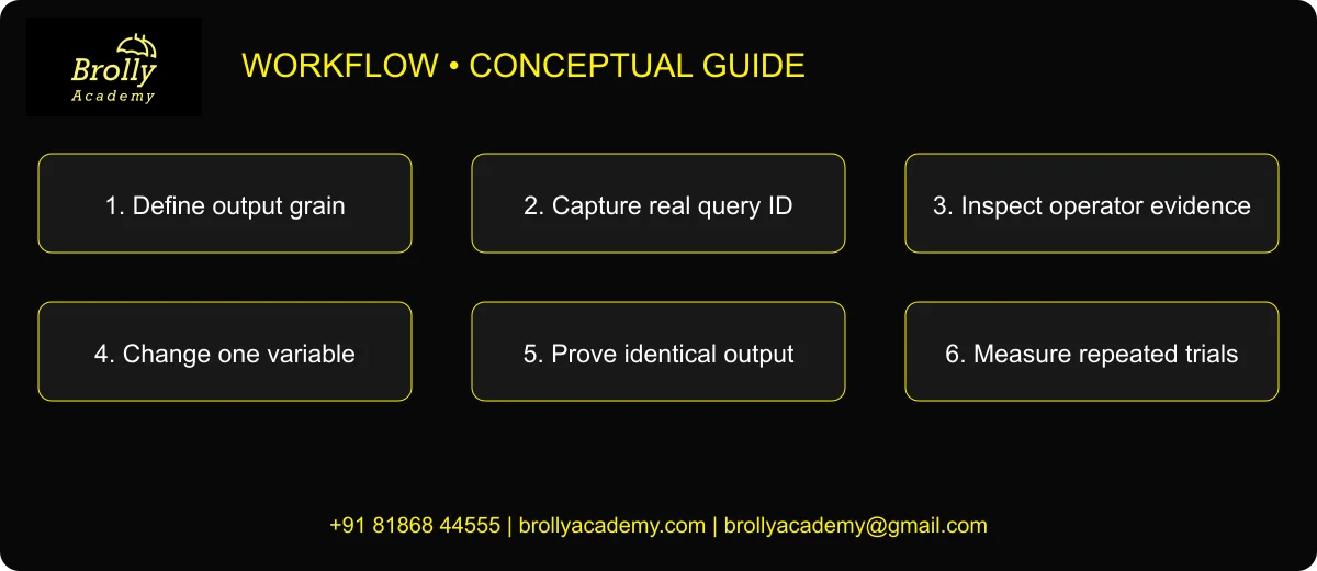
- Run A and B repeatedly in alternating order. Use a small fixed number of trials that fits your budget and capture every query ID.
- Separate first-run provisioning/cold behavior from later warm-cache behavior. USE_CACHED_RESULT=FALSE does not turn off all caches.
- Record execution time, total elapsed time, queue time, scan volume, partition counts and spill. Compare the metric connected to the diagnosed bottleneck.
- Keep an experiment log with actual observations. If timing differences are tiny or inconsistent, report no demonstrated improvement rather than selecting the single fastest run.
| Version | Query ID | Execution ms | Queue ms | Partitions scanned/total | Result check |
|---|---|---|---|---|---|
| Baseline A1 | Record actual ID | Measure | Measure | Measure | Pass/fail |
| Candidate B1 | Record actual ID | Measure | Measure | Measure | Pass/fail |
| Further alternating trials | Record each ID | Measure | Measure | Measure | Pass/fail |
This table is a measurement worksheet, not a claimed benchmark. You can calculate median and range from recorded runs, but keep concurrency, warehouse changes and any failed validation visible. Faster execution can coexist with higher resource use; a credit-saving claim needs an appropriate cost measurement, not elapsed time alone.
10. Diagnose exploding joins and memory spill separately
Before any large join, establish the key contract. The following read-only check identifies duplicate dimension keys:
SELECT customer_id,COUNT(*) AS copies FROM DIM_CUSTOMER
GROUP BY customer_id HAVING COUNT(*)>1;
SELECT COUNT(*) AS joined_rows
FROM FACT_ORDER f JOIN DIM_CUSTOMER c USING(customer_id);
For the seed dataset, joined_rows should equal 100,000. If it increases unexpectedly, inspect the relationship. Do not add DISTINCT to hide the problem: identical amounts or events can make that drop legitimate rows. A business-approved current-customer view may be needed, but a changing dimension requires explicit effective-date logic.
Spill means an operator required more working space than available memory and used storage. First inspect how much data reaches the operator. Reduce unused columns, unnecessary intermediate rows or a mistaken join expansion. Then evaluate whether warehouse sizing is justified. Do not assume multi-cluster concurrency scaling supplies more memory to one running query.
Reference: Queries too large to fit in memory.
11. Choose optional physical optimizations from evidence
| Option | Question before adopting | Validation |
|---|---|---|
| Warehouse size | Is the query compute/memory bound, and does added capacity improve the relevant objective? | Compare workload results, latency and usage under controlled conditions |
| Clustering key | Do repeated selective predicates suffer from poor pruning on a sufficiently large table? | Inspect partition evidence and maintenance cost |
| Search optimization | Is the workload an eligible selective lookup pattern? | Verify support, selectivity and ongoing service cost |
| Materialized result strategy | Is expensive work repeated at an acceptable freshness boundary? | Measure refresh cost, correctness and stale-data tolerance |
| Concurrency design | Is queueing caused by simultaneous demand? | Compare queue metrics and user workload isolation |
These are evaluation options, not changes enabled by this exercise. Avoid applying all of them at once; that prevents attribution and can add ongoing spend. An optimization valid for a dashboard point lookup may be irrelevant to a full-month aggregate.
Review the official performance guide for feature-specific investigations. For a refreshed downstream SQL table, use the separate Dynamic Tables walkthrough instead of silently changing this query lab into a pipeline tutorial.
12. Troubleshoot, restore the session and present your evidence
| Problem | Check | Next action |
|---|---|---|
| No profile found | Actual SELECT ID, execution completion, permissions and age | Use a recent own-query ID and documented access |
| A/B outputs differ | Date boundaries, join grain, NULL handling and changed seed | Fix semantics before comparing speed |
| Candidate is not faster | Small dataset, optimizer-equivalent plan or added aggregation | Keep baseline if evidence does not support the rewrite |
| History looks incomplete | Session scope, result limit and query IDs | Filter the recent correct session and capture IDs immediately |
| Unexpectedly fast repeated run | Persisted result reuse and warehouse data cache | Label the cache state and rerun the intended experiment |
Restore USE_CACHED_RESULT and QUERY_TAG to the values recorded in section 3. If the original tag was unset, use UNSET; otherwise restore its original string. The example below applies only when the original cache flag was TRUE and the original tag was unset:
ALTER SESSION SET USE_CACHED_RESULT=TRUE;
ALTER SESSION UNSET QUERY_TAG;
-- After saving evidence, remove only the disposable lab:
DROP SCHEMA BA_QO_LAB;
Keep setup.sql, baseline.sql, candidate.sql, validation.sql, query-ids.csv and a README describing the workload, hypothesis, parameters and actual results. A useful interview explanation is: “I checked join uniqueness, captured both report IDs, compared operator evidence, proved region-level equivalence and measured repeated trials.” Do not claim a percentage improvement unless the saved experiment supports it.
Continue with Snowflake Projects for portfolio ideas, interview questions for explaining tradeoffs, or the Snowflake course syllabus for structured learning.
13. Snowflake query optimization FAQs
What should I check first for a slow Snowflake query?
Identify whether time is spent compiling, queueing or executing. Then inspect the relevant operators and validate the business result before changing SQL.
Does a larger warehouse always solve slow queries?
No. It does not correct duplicate joins, unnecessary work or every compilation problem. Test capacity changes against the actual bottleneck and budget.
Does USE_CACHED_RESULT=FALSE clear every cache?
No. It controls persisted query-result reuse for the session; warehouse data caching and provisioning state still affect the experiment.
Are CTEs always slower than subqueries?
No universal rule applies. Inspect the plan and compare equivalent results. The optimizer and reference pattern determine the work performed.
Why use a half-open date range?
It states the lower inclusive and upper exclusive boundaries clearly. That avoids guessing the final timestamp of a month. Actual pruning still needs inspection.
Why can pre-aggregation help a join?
It can reduce rows reaching the join when the required grain allows it. It also adds work and requires correct dimension uniqueness, so validate and measure.
How do I recognize an exploding join?
Compare input and output rows with the intended relationship. Investigate missing predicates or duplicate keys instead of hiding unexpected rows with DISTINCT.
What does remote spill indicate?
An operator used storage after exceeding available working memory. Inspect the intermediate data and relevant capacity; do not assume any spill proves the same fix is needed.
Can I prove equivalence with a total alone?
No. Equal totals can hide values assigned to the wrong region. Use two-way differences plus uniqueness checks at the required output grain.
Is the 100,000-row lab a production benchmark?
No. It is a deterministic correctness and profiling exercise. Larger production claims require representative data, concurrency and repeated controlled measurements.
Should I enable clustering for every table?
No. Evaluate repeated predicate patterns, pruning evidence, table scale and maintenance cost before selecting a key or enabling a service.
Were the timing results measured in Snowflake?
No connected Snowflake execution was performed. The article supplies expected logical outputs and an experiment procedure; fill in real query IDs and timings from your own run.
Open the phase-by-phase SQL workbook. Read each phase in context; do not execute the complete workbook as one batch.
Related Snowflake Articles
Snowflake Projects
Choose a portfolio exercise with SQL, expected results and validation steps.
Snowflake Interview Questions
Practise explaining SQL, validation and project decisions.
Snowflake Certification
Explore the separate certification learning path and exam preparation.
Related Courses
Snowflake Training
Explore the syllabus, practical learning topics and available Snowflake training formats.
Azure Data Factory Training
Explore data integration, orchestration and cloud pipeline training.