Data Science Projects Ideas

Top 100+ Data Science Projects Ideas with Source Code

Are you looking for high-impact data science projects to boost your resume or gain real-world skills in 2025? This comprehensive guide presents over 100 data science project ideas, ranging from beginner to advanced levels, across various domains and technologies. Each project includes problem statements, datasets, tools, and expected outcomes to help you practice effectively and build a job-ready portfolio.

Whether you’re just getting started or seeking to sharpen your expertise, these projects offer valuable hands-on experience with real-world data, modern tools, and industry practices. From machine learning to natural language processing and computer vision, this list is designed to help you grow as a data scientist in a structured and impactful way.

What Is Data Science?

Data science is a multidisciplinary field that combines mathematics, statistics, computer science, and domain expertise to analyze and interpret large volumes of data. It is a core component of data-driven decision-making in modern businesses and organizations.

A Typical Data Science Workflow Involves:

Data Collection and Cleaning: Acquiring raw data and preparing it for analysis
Exploratory Data Analysis (EDA): Discovering trends, patterns, and anomalies
Statistical Modelling and Machine Learning: Developing algorithms for predictions or classification
Data Visualization and Storytelling: Communicating insights through dashboards, charts, or reports
Predictive and Prescriptive Analytics: Forecasting future outcomes and suggesting actions

Data science is widely used in industries such as finance, healthcare, e-commerce, marketing, logistics, and cybersecurity. Common applications include fraud detection, customer segmentation, sales forecasting, recommendation systems, and churn prediction.

Why Work on Data Science Projects?

Building data science projects is one of the most effective ways to transition from theory to practice. Here’s why working on projects is crucial for every data science learner or professional:

1. Apply Theoretical Knowledge

Projects help you move beyond classroom concepts and apply machine learning algorithms, statistical techniques, and data handling skills in real-life contexts.

2. Master Industry Tools

By working on projects, you gain hands-on experience with essential tools and libraries such as:

Programming Languages: Python, R
Libraries: Pandas, NumPy, Scikit-learn, Matplotlib, Seaborn, TensorFlow
Data Visualization Tools: Power BI, Tableau
Database Technologies: SQL, NoSQL

This experience directly translates to the skill sets required in professional roles.

3. Build a Portfolio That Stands Out

Publishing your projects on platforms like GitHub allows you to showcase your work to potential employers. A strong portfolio demonstrates initiative, capability, and practical experience.

4. Prepare for Job Interviews and Case Studies

Many companies assess candidates based on their project experience. Being able to discuss your process—from data acquisition to model evaluation—can give you a competitive advantage in technical interviews.

5. Strengthen Problem-Solving Skills

Each project challenges you to define problems, test hypotheses, build models, and evaluate results. This iterative process develops your analytical thinking, a vital skill in any data-driven role.

Who Should Use These Project Ideas?

These projects are ideal for:

Students working on academic assignments or final-year projects
Job seekers preparing for roles in data science, machine learning, or analytics
Aspiring data scientists looking to build a practical foundation
Working professionals transitioning into data-driven roles

Instructors and mentors designing project-based learning experiences

Beginner-Level Data Science Project Ideas

Basic EDA Projects

1. Titanic Survival Prediction

(Binary Classification using Logistic Regression, Decision Trees)

Objective

Predict whether a passenger survived the Titanic disaster based on features like age, sex, class, and fare.

Dataset Source

Kaggle Titanic Dataset

Techniques

Missing value imputation
Label encoding (Sex, Embarked)
Logistic Regression, Decision Tree, Random Forest
Evaluation: Accuracy, ROC-AUC, Confusion Matrix

Key Features

Pclass, Sex, Age, SibSp, Parch, Fare, Embarked

Tools

Python, pandas, scikit-learn, seaborn, matplotlib

Sample Code Snippet

python

				
					from sklearn.linear_model import LogisticRegression
from sklearn.model_selection import train_test_split
import pandas as pd

df = pd.read_csv('titanic.csv')
df['Sex'] = df['Sex'].map({'male': 0, 'female': 1})
df['Age'].fillna(df['Age'].median(), inplace=True)

X = df[['Pclass', 'Sex', 'Age', 'Fare']]
y = df['Survived']
X_train, X_test, y_train, y_test = train_test_split(X, y)

model = LogisticRegression()
model.fit(X_train, y_train)
print("Accuracy:", model.score(X_test, y_test))

2. Iris Flower Classification

(Multi-class Classification using SVM, KNN, Decision Trees)

Objective

Classify iris flowers into three species based on petal and sepal measurements.

Dataset Source

UCI ML Repository: Iris Dataset

Techniques

Exploratory Data Analysis
Support Vector Machines, K-Nearest Neighbors, Decision Tree
Cross-validation for performance

Key Features

SepalLength, SepalWidth, PetalLength, PetalWidth

Tools

Python, scikit-learn, seaborn, matplotlib

Sample Code Snippet

				
					from sklearn.datasets import load_iris
from sklearn.tree import DecisionTreeClassifier
from sklearn.model_selection import train_test_split

iris = load_iris()
X_train, X_test, y_train, y_test = train_test_split(iris.data, iris.target)

model = DecisionTreeClassifier()
model.fit(X_train, y_train)
print("Model accuracy:", model.score(X_test, y_test))

3. Netflix Top 10 Analysis

(EDA and Trend Analysis Project)

Objective

Analyze trending content on Netflix to uncover patterns in content type, country distribution, and weekly views.

Dataset Source

Netflix Top 10 Titles (via Kaggle or top10.netflix.com)

Techniques

Time series aggregation
Genre and country breakdown
Barcharts, line graphs, heatmaps
Optional: Tableau or Power BI dashboard

Key Features

Title, Week, Views, Category, Country

Tools

Python (pandas, seaborn), Tableau, or Power BI

Sample Code Snippet

				
					import pandas as pd
import seaborn as sns
import matplotlib.pyplot as plt

df = pd.read_csv('netflix_top10.csv')
top_titles = df['title'].value_counts().head(10)

plt.figure(figsize=(10, 6))
sns.barplot(x=top_titles.values, y=top_titles.index)
plt.title("Most Frequent Netflix Top 10 Titles")
plt.xlabel("Weeks in Top 10")
plt.show()

4. Google Play Store Review Analysis

(NLP Sentiment Classification Project)

Objective

Analyze user reviews to identify sentiment and common issues in apps listed on the Google Play Store.

Dataset Source

Google Play Store Apps Dataset (Kaggle)

Techniques

Text preprocessing (cleaning, tokenizing)
TF-IDF vectorization
Sentiment prediction using Naive Bayes / Logistic Regression
Word cloud for keywords

Key Features

App Name, Review Text, Sentiment, Rating

Tools

Python, NLTK, scikit-learn, WordCloud

Sample Code Snippet

				
					from sklearn.feature_extraction.text import TfidfVectorizer
from sklearn.naive_bayes import MultinomialNB
from sklearn.model_selection import train_test_split

df = pd.read_csv('playstore_reviews.csv')
df = df.dropna(subset=['Translated_Review', 'Sentiment'])

vectorizer = TfidfVectorizer(stop_words='english')
X = vectorizer.fit_transform(df['Translated_Review'])
y = df['Sentiment'].map({'Positive': 1, 'Negative': 0, 'Neutral': 2})

X_train, X_test, y_train, y_test = train_test_split(X, y)
model = MultinomialNB()
model.fit(X_train, y_train)
print("Accuracy:", model.score(X_test, y_test))

5. Airbnb Price Prediction (Basic Regression Project)

Objective

Predict Airbnb listing prices based on room features, location, availability, and ratings.

Dataset Source

Techniques

Data cleaning and missing value handling
Feature encoding (neighborhood, room type)
Linear Regression or XGBoost
Evaluation: MAE, RMSE

Key Features

Room Type, Reviews, Availability, Location, Amenities

Tools

Python, pandas, scikit-learn, seaborn

Sample Code Snippet

				
					from sklearn.linear_model import LinearRegression
from sklearn.model_selection import train_test_split

df = pd.read_csv('airbnb_nyc.csv')
df = df[df['price'] < 500]  # Remove outliers
df['room_type'] = df['room_type'].astype('category').cat.codes

X = df[['room_type', 'minimum_nights', 'number_of_reviews']]
y = df['price']

X_train, X_test, y_train, y_test = train_test_split(X, y)
model = LinearRegression()
model.fit(X_train, y_train)
print("Model R^2 Score:", model.score(X_test, y_test))

Python & Pandas Projects

Project 1 : Weather Data Analysis

Problem Statement

Weather patterns impact everything from agriculture to logistics. Analyzing weather trends helps in forecasting and planning across sectors.

Objective

Analyze weather data to identify temperature patterns, precipitation trends, seasonal changes, and potential anomalies.

Dataset Source

Key Analysis Areas

Daily/Monthly average temperature trends
Heatmaps of temperature and rainfall by region
Extreme weather event detection
Year-over-year comparison

Tools Used

Python (Pandas, Seaborn, Matplotlib), Tableau, Power BI

Expected Outcome

Visual and statistical insights into climate patterns that can inform decision-making for agriculture, energy, and public safety.

Sample Use Case

“How has the average temperature changed over the last 20 years in New Delhi?”

1. Weather Data Analysis – Sample Code Snippet

				
					import pandas as pd
import matplotlib.pyplot as plt
import seaborn as sns

# Load dataset
df = pd.read_csv('weather_data.csv')  # columns: Date, City, Temperature, Precipitation

# Convert date column
df['Date'] = pd.to_datetime(df['Date'])
df['Month'] = df['Date'].dt.month

# Monthly average temperature
monthly_avg = df.groupby('Month')['Temperature'].mean()

# Plot
plt.figure(figsize=(10, 5))
sns.lineplot(x=monthly_avg.index, y=monthly_avg.values)
plt.title('Monthly Average Temperature')
plt.xlabel('Month')
plt.ylabel('Temperature (°C)')
plt.grid()
plt.show()

Project 2 : COVID-19 Data Tracker

Problem Statement

Tracking the spread of COVID-19 helps in evaluating the effectiveness of public health policies and predicting future outbreaks.

Objective

Create a dynamic dashboard to monitor COVID-19 cases, deaths, and recoveries over time and across regions.

Dataset Source

Johns Hopkins CSSE COVID-19 Data
Our World in Data COVID-19 Dataset

Key Analysis Areas

Daily case and death trends
Vaccination progress
Country-wise and state-wise heatmaps
Case fatality rate and recovery trends

Tools Used

Power BI, Tableau, Python (Plotly, Dash), Excel

Expected Outcome

An interactive dashboard for public use or internal reporting, highlighting trends and hotspot zones.

Sample Use Case

“Track India’s vaccination progress compared to global averages.”

2. COVID-19 Data Tracker – Sample Code Snippet

				
					import pandas as pd
import matplotlib.pyplot as plt

# Load dataset
df = pd.read_csv('covid19_data.csv')  # columns: date, country, confirmed, deaths, recovered

# Filter country
india = df[df['country'] == 'India']
india['date'] = pd.to_datetime(india['date'])

# Plot daily cases
plt.figure(figsize=(10, 5))
plt.plot(india['date'], india['confirmed'], label='Confirmed Cases')
plt.plot(india['date'], india['deaths'], label='Deaths')
plt.title('COVID-19 Daily Cases in India')
plt.xlabel('Date')
plt.ylabel('Number of Cases')
plt.legend()
plt.tight_layout()
plt.show()

Project 3: Global Terrorism Dataset Analysis

Problem Statement

Understanding global terrorism patterns helps governments and researchers identify high-risk regions and develop prevention strategies.

Objective

Explore terrorism data to analyze attack frequency, types, locations, casualties, and group activities over time.

Dataset Source

Key Analysis Areas

Top countries and regions by number of attacks
Attack type distribution (bombing, armed assault, etc.)
Year-wise casualties and fatalities
Active terrorist groups and their target types

Tools Used

Python (Pandas, Seaborn), Tableau, Power BI, GeoPandas for maps

Expected Outcome

An analytical report or dashboard that helps visualize global threat trends, target types, and geographical hotspots.

Sample Use Case

“Which countries saw the highest number of terrorism incidents in the past decade?”

3. Global Terrorism Dataset Analysis – Sample Code Snippet

				
					import pandas as pd
import seaborn as sns
import matplotlib.pyplot as plt

# Load dataset
df = pd.read_csv('global_terrorism.csv')  # columns: country_txt, attacktype1_txt, nkill, iyear

# Top 10 countries by attacks
top_countries = df['country_txt'].value_counts().head(10)

# Plot
plt.figure(figsize=(10, 6))
sns.barplot(x=top_countries.values, y=top_countries.index)
plt.title('Top 10 Countries by Terrorist Attacks')
plt.xlabel('Number of Attacks')
plt.ylabel('Country')
plt.show()

Project 4: FIFA World Cup Data Exploration

Problem Statement

Football analysts and fans are always curious about historical team and player performances, winning strategies, and match statistics.

Objective

Explore historical FIFA World Cup data to extract insights on top scorers, team performance, goal trends, and match outcomes.

Dataset Source

Key Analysis Areas

Most goals by team and player
Match outcome breakdown (win/loss/draw)
Country performance over the years
Goal distribution by stage (group vs knockout)

Tools Used

Python, Tableau, Excel, Power BI

Expected Outcome

An engaging analytical dashboard for fans, journalists, or sports data scientists to analyze team strengths and historical records.

Sample Use Case

“Which team has the highest goal average per tournament in FIFA history?”

FIFA World Cup Data Exploration – Sample Code Snippet

				
					import pandas as pd
import seaborn as sns
import matplotlib.pyplot as plt

# Load dataset
matches = pd.read_csv('fifa_world_cup_matches.csv')  # columns: year, home_team, away_team, home_score, away_score

# Calculate total goals per match
matches['total_goals'] = matches['home_score'] + matches['away_score']

# Plot average goals by year
avg_goals = matches.groupby('year')['total_goals'].mean()

plt.figure(figsize=(10, 5))
sns.lineplot(x=avg_goals.index, y=avg_goals.values)
plt.title('Average Goals per Match by Year')
plt.xlabel('Year')
plt.ylabel('Average Goals')
plt.grid()
plt.show()

Project 5 : Olympics Dataset Insights

Problem Statement

The Olympics host thousands of athletes, yet countries and athletes differ significantly in performance and participation trends.

Objective

Explore historical Olympics data to discover medal trends, country-wise dominance, athlete participation, and sport popularity.

Dataset Source

Olympics Dataset (Kaggle)

Key Analysis Areas

Total medals by country
Gender-wise participation trends
Dominant sports by nation
Medal distribution over time

Tools Used

Power BI, Tableau, Python (Seaborn, Matplotlib)

Expected Outcome

A full analytical report or interactive dashboard that showcases global sports trends, equity in participation, and medal dominance.

Sample Use Case

“Which countries have shown the fastest growth in medal wins over the last 5 Olympic events?”

Olympics Dataset Insights – Sample Code Snippet

				
					import pandas as pd
import seaborn as sns
import matplotlib.pyplot as plt

# Load dataset
df = pd.read_csv('olympics.csv')  # columns: Year, Country, Medal

# Filter only medal records
medals = df[df['Medal'].notnull()]

# Group by country
top_countries = medals['Country'].value_counts().head(10)

# Plot
plt.figure(figsize=(10, 6))
sns.barplot(x=top_countries.values, y=top_countries.index)
plt.title('Top 10 Countries by Total Olympic Medals')
plt.xlabel('Medal Count')
plt.ylabel('Country')
plt.show()

Data Visualization Projects

Project 1: Sales Dashboard in Tableau

Problem Statement

Sales leaders need real-time visibility into regional, category-wise, and monthly sales to drive revenue and decision-making.

Objective

Create an interactive Tableau dashboard to monitor sales performance, trends, and KPIs like revenue, profit margin, and sales growth.

Dataset Source

Superstore Sales Dataset (Kaggle / Tableau Public)

Key Features

Filters for category, region, and date
KPIs: Total Sales, Profit, Quantity, Discount
Line chart for trend analysis
Geo map for state-wise sales
Bar chart for top-performing products

Tools Used

Tableau Desktop or Tableau Public

Outcome

An executive-ready dashboard for identifying underperforming regions, forecasting growth, and making data-driven decisions.

Video Tutorial Suggestions

“Build a Sales Dashboard in Tableau – Step by Step”
“Superstore Analysis with Filters and KPIs”

Project 2: Indian Startup Funding Analysis

Problem Statement

Investors and analysts want to understand startup trends in India: funding size, sector growth, and location-wise investment patterns.

Objective

Create a dashboard to visualize startup funding trends in India across sectors, cities, and time.

Dataset Source

Indian Startup Funding Dataset (Kaggle)

Key Features

Total Funding Raised by Year
Sector-wise and City-wise Investment Distribution
Funding Trends Over Time
Top Funded Startups

Tools Used

Tableau or Power BI, Excel, Python (optional preprocessing)

Outcome

A complete visual analytics dashboard to explore startup ecosystem insights, ideal for VCs, analysts, or journalists.

Video Tutorial Suggestions

“Startup Funding Dashboard using Power BI or Tableau”
“Top 10 Funded Startups Visualisation”

Project 3 : YouTube Trending Video Analytics

Problem Statement

Content creators and digital marketers want to decode trends and audience behavior from YouTube’s trending videos.

Objective

Analyze YouTube trending video datasets to find common traits in viral content—views, tags, likes/dislikes ratio, category performance.

Dataset Source

YouTube Trending Videos Dataset (Kaggle)

Key Features

Views vs. Likes ratio
Trending Video Category Breakdown
Word Clouds for Common Tags
Publishing Time Analysis (hour/day of week)

Tools Used

Tableau, Power BI, or Python (Seaborn + Plotly Dash for interactive dashboards)

Outcome

A dashboard revealing what makes videos trend—valuable for content strategy, SEO, and YouTube campaign planning.

Video Tutorial Suggestions

“YouTube Data Analysis with Tableau or Power BI”
“Viral Video Analytics Dashboard Walkthrough”

Project 4 : IPL Scorecard Analysis Using Power BI

Problem Statement

Cricket enthusiasts and sports analysts need deeper insights into player performance, team stats, and match outcomes across IPL seasons.

Objective

Build an IPL dashboard in Power BI showing season stats, batting and bowling performance, win/loss ratios, and player comparisons.

Dataset Source

IPL Matches & Deliveries Dataset (Kaggle)

Key Features

Player Run/Strike Rate Charts
Team Win Ratios by Season
Toss Impact vs. Match Result
Most Runs/Wickets Leaderboard
Filters: team, player, season

Tools Used

Power BI Desktop, DAX, Power Query

Outcome

An interactive cricket analytics dashboard suitable for presentation to media, fans, or cricket boards.

Video Tutorial Suggestions

“IPL Dashboard in Power BI with DAX”
“Match Stats and Player Analysis in Power BI”

Project 5 : Indian Census Visualization

Problem Statement

Policy-makers and researchers need a simple way to understand population demographics, literacy rates, and gender distribution across Indian states.

Objective

Visualize key census indicators using charts, maps, and filters for state/district-level data.

Dataset Source

India Census 2011 Dataset (data.gov.in)

Key Features

State-wise Population Pyramid
Literacy Rate Heatmap
Gender Ratio by District
Urban vs. Rural Population Distribution

Tools Used

Tableau or Power BI with shapefiles for map visualizations

Outcome

An informative dashboard that supports demographic research, policy making, and public data storytelling.

Video Tutorial Suggestions

“Building Indian Census Dashboard with Tableau Maps”
“Visualizing Census Data with Power BI and Excel”

Intermediate-Level Data Science Project Ideas

Supervised Learning Projects

Project 1: Credit Card Default Prediction

Problem Statement

Financial institutions must assess the risk of loan or credit card default to minimize losses and improve lending strategies.

Objective

Build a classification model to predict whether a customer is likely to default on their credit card payment.

Dataset Source

Techniques and Concepts

Binary classification
Feature engineering (repayment history, credit utilization)
Handling class imbalance (SMOTE, undersampling)
Logistic Regression, Random Forest, XGBoost

Tools and Libraries

Python, pandas, scikit-learn, imbalanced-learn, matplotlib, XGBoost

Expected Outcome

A model with performance metrics like AUC-ROC, precision-recall that helps banks proactively manage high-risk clients.

Sample Code Snippet

				
					from sklearn.model_selection import train_test_split
from sklearn.ensemble import RandomForestClassifier
from sklearn.metrics import classification_report

data = pd.read_csv("credit_card_default.csv")
X = data.drop("default", axis=1)
y = data["default"]

X_train, X_test, y_train, y_test = train_test_split(X, y, test_size=0.2)
model = RandomForestClassifier()
model.fit(X_train, y_train)

preds = model.predict(X_test)
print(classification_report(y_test, preds))

Project 2 : Diabetes Prediction Using Machine

Problem Statement

Early detection of diabetes can significantly reduce the impact of the disease, especially in high-risk populations.

Objective

Develop a model that predicts the presence of diabetes based on diagnostic health parameters.

Dataset Source

Pima Indians Diabetes Dataset (UCI)

Techniques and Concepts

Binary classification
Feature scaling and outlier treatment
Logistic Regression, SVM, Decision Trees
Evaluation using accuracy, recall, F1-score

Tools and Libraries

Python, pandas, scikit-learn, seaborn, matplotlib

Expected Outcome

A prediction model usable by healthcare providers to flag potential diabetes cases early.

Sample Code Snippet

				
					from sklearn.preprocessing import StandardScaler
from sklearn.linear_model import LogisticRegression
from sklearn.metrics import accuracy_score

df = pd.read_csv("diabetes.csv")
X = df.drop("Outcome", axis=1)
y = df["Outcome"]

scaler = StandardScaler()
X_scaled = scaler.fit_transform(X)

model = LogisticRegression()
model.fit(X_scaled, y)

print("Accuracy:", model.score(X_scaled, y))

Project 3 : House Price Prediction (Advanced Regression)

Problem Statement

Home buyers and real estate businesses need accurate house price estimations to make informed buying, selling, and investment decisions.

Objective

Predict housing prices based on features such as location, square footage, number of rooms, and amenities.

Dataset Source

Kaggle House Prices: Advanced Regression Challenge

Techniques and Concepts

Regression modeling
Missing value treatment and one-hot encoding
Feature selection and cross-validation
XGBoost, Lasso Regression, Ridge Regression

Tools and Libraries

Python, pandas, numpy, scikit-learn, XGBoost, LightGBM

Expected Outcome

An accurate regression model with RMSE as the performance metric, usable for dynamic price estimation apps.

Sample Code Snippet

				
					from sklearn.model_selection import cross_val_score
from xgboost import XGBRegressor

data = pd.read_csv("house_prices.csv")
X = data.drop(["SalePrice", "Id"], axis=1)
y = data["SalePrice"]

model = XGBRegressor()
scores = cross_val_score(model, X, y, scoring='neg_root_mean_squared_error', cv=5)
print("Average RMSE:", -scores.mean())

Project 4 : Email Spam Detection

Problem Statement

Email service providers need to identify and filter spam emails without blocking important user messages.

Objective

Classify emails as spam or not spam based on their content, metadata, and structure.

Dataset Source

Techniques and Concepts

Natural Language Processing (NLP)
Text preprocessing (tokenization, stopword removal, TF-IDF)
Naive Bayes, Logistic Regression, SVM
Evaluation using confusion matrix and ROC-AUC

Tools and Libraries

Python, scikit-learn, NLTK, pandas, seaborn

Expected Outcome

A lightweight spam detection engine that can be deployed in real-time email systems.

Sample Code Snippet

				
					from sklearn.feature_extraction.text import TfidfVectorizer
from sklearn.naive_bayes import MultinomialNB

data = pd.read_csv("spam.csv")
X = data["message"]
y = data["label"].map({"ham":0, "spam":1})

tfidf = TfidfVectorizer()
X_vec = tfidf.fit_transform(X)

model = MultinomialNB()
model.fit(X_vec, y)

print("Spam detection accuracy:", model.score(X_vec, y))

Project 5: Heart Disease Risk Classifier

Problem Statement

Cardiovascular disease is a leading cause of death globally. Predictive models can save lives by enabling early diagnosis.

Objective

Predict the likelihood of a patient having heart disease based on diagnostic features such as age, cholesterol, and resting ECG.

Dataset Source

UCI Heart Disease Dataset

Techniques and Concepts

Binary classification
Data normalization and correlation filtering
Logistic Regression, Random Forest, KNN
Precision-recall and ROC curve analysis

Tools and Libraries

Python, pandas, seaborn, scikit-learn, matplotlib

Expected Outcome

A clinically useful model for screening high-risk patients using routine medical data.

Sample Code Snippet

				
					from sklearn.model_selection import train_test_split
from sklearn.ensemble import RandomForestClassifier

df = pd.read_csv("heart.csv")
X = df.drop("target", axis=1)
y = df["target"]

X_train, X_test, y_train, y_test = train_test_split(X, y, test_size=0.3)
model = RandomForestClassifier()
model.fit(X_train, y_train)

print("Test Accuracy:", model.score(X_test, y_test))

Unsupervised Learning Projects

Clustering Project 1: Customer Segmentation Using K-Means

Problem Statement

Businesses struggle to personalize marketing and product strategies for diverse customer bases. A one-size-fits-all approach reduces engagement and retention.

Objective

Group customers based on purchasing behavior, demographics, and activity using K-Means Clustering to enable targeted marketing strategies.

Dataset Source

Mall Customer Segmentation Dataset (Kaggle)
Retail CRM export files or e-commerce user logs

Techniques and Concepts

Data normalization (MinMaxScaler, StandardScaler)
Elbow method and silhouette score for optimal k
K-Means clustering
PCA for visualization of clusters

Tools and Libraries

Python, pandas, scikit-learn, matplotlib, seaborn, plotly

Expected Outcome

Visual cluster groups that help businesses identify high-value customers, discount seekers, or infrequent shoppers for campaign targeting.

Sample Code Snippet

				
					from sklearn.cluster import KMeans
from sklearn.preprocessing import StandardScaler
import pandas as pd
import matplotlib.pyplot as plt

data = pd.read_csv("Mall_Customers.csv")
features = data[['Annual Income (k$)', 'Spending Score (1-100)']]

scaler = StandardScaler()
scaled_features = scaler.fit_transform(features)

kmeans = KMeans(n_clusters=5)
kmeans.fit(scaled_features)
data['Cluster'] = kmeans.labels_

plt.scatter(scaled_features[:, 0], scaled_features[:, 1], c=kmeans.labels_)
plt.title('Customer Segments')
plt.show()

Video Tutorial Suggestions

“K-Means Clustering from Scratch in Python“
“Customer Segmentation with Mall Dataset”
“How to Choose Optimal Clusters Using Elbow Method”

Clustering Project 2 : Movie Genre Clustering

Problem Statement

Streaming platforms need to understand movie similarity and genre overlap to improve recommendations and navigation.

Objective

Cluster movies based on metadata (tags, synopsis, cast, ratings) to find similar titles or hidden genre combinations.

Dataset Source

Techniques and Concepts

Text vectorization (TF-IDF on synopsis)
Feature encoding (genres, ratings, runtime)
Dimensionality reduction (PCA, t-SNE)
K-Means, Hierarchical Clustering

Tools and Libraries

Python, scikit-learn, pandas, NLTK, spaCy, plotly

Expected Outcome

A genre clustering system that shows which movies are similar based on storyline, cast, and themes — useful for content-based filtering.

Sample Code Snippet

				
					from sklearn.feature_extraction.text import TfidfVectorizer
from sklearn.cluster import KMeans
import pandas as pd

movies = pd.read_csv("tmdb_5000_movies.csv")
tfidf = TfidfVectorizer(stop_words='english')
synopsis_matrix = tfidf.fit_transform(movies['overview'])

model = KMeans(n_clusters=10)
model.fit(synopsis_matrix)
movies['Cluster'] = model.labels_

Video Tutorial Suggestions

“Movie Clustering Using TF-IDF and KMeans”
“Unsupervised Learning for Recommender Systems”
“Genre Detection with NLP and Clustering”

Clustering Project 3 : Market Basket Analysis

Problem Statement

Retailers want to understand which items are frequently purchased together to optimize product placement, bundling, and promotions.

Objective

Identify item associations and clusters in transactional data using association rules and clustering.

Dataset Source

Groceries Dataset (Kaggle)
Instacart Market Basket Data

Techniques and Concepts

Apriori algorithm for association rules
Itemset frequency filtering
K-Modes or DBSCAN for categorical clustering
Lift, confidence, and support metrics

Tools and Libraries

Python, mlxtend, pandas, seaborn, matplotlib

Expected Outcome

Association rules like “If a customer buys milk, they are likely to buy bread,” and product clusters for bundle offers.

Sample Code Snippet

				
					from mlxtend.frequent_patterns import apriori, association_rules
import pandas as pd

data = pd.read_csv("groceries.csv")
basket = data.groupby(['Member_number', 'itemDescription'])['itemDescription'].count().unstack().fillna(0)
basket = basket.applymap(lambda x: 1 if x > 0 else 0)

frequent_itemsets = apriori(basket, min_support=0.02, use_colnames=True)
rules = association_rules(frequent_itemsets, metric='lift', min_threshold=1)
print(rules[['antecedents', 'consequents', 'support', 'confidence', 'lift']])

Video Tutorial Suggestions

“Market Basket Analysis with Python”
“Apriori and Association Rules in Retail”
“Visualizing Product Clusters from Transaction Logs”

Clustering Project 4 : Crime Rate Clustering in Indian States

Problem Statement

Law enforcement and policy-makers need to analyze regional crime trends to allocate resources, enhance security, and monitor high-risk zones.

Objective

Cluster Indian states based on crime rates across various categories like theft, assault, and cybercrime using unsupervised learning.

Dataset Source

Techniques and Concepts

Feature normalization
K-Means or Agglomerative Clustering
Heatmaps and cluster maps for visualization
Interpretation of regional crime patterns

Tools and Libraries

Python, pandas, seaborn, scikit-learn, geopandas (for maps)

Expected Outcome

Interactive visualizations and clusters showing which Indian states have similar crime profiles for decision-making and policing.

Sample Code Snippet

				
					import pandas as pd
from sklearn.preprocessing import StandardScaler
from sklearn.cluster import KMeans
import seaborn as sns

df = pd.read_csv("crime_india.csv")
features = df[['Murder', 'Theft', 'Cybercrime', 'Rape']]
scaled = StandardScaler().fit_transform(features)

kmeans = KMeans(n_clusters=4)
df['Cluster'] = kmeans.fit_predict(scaled)

sns.heatmap(df.groupby('Cluster').mean(), cmap='Reds', annot=True)

Video Tutorial Suggestions

“Crime Clustering by State using KMeans”
“Unsupervised Learning for Government Analytics”
“Visualizing Crime Patterns in Indian States”

Time Series Forecasting Projects

Time Series Project 1 : Stock Price Prediction

Problem Statement

Investors and financial institutions require reliable models to forecast stock prices for decision-making, risk management, and portfolio optimization.

Objective

Build a model that predicts future stock prices using historical price trends and market indicators.

Dataset Source

Techniques and Concepts

Time series analysis and decomposition
Moving averages, RSI, Bollinger Bands
ARIMA, SARIMA, Prophet
LSTM or GRU for deep learning time series models

Tools and Libraries

Python, yfinance, pandas, matplotlib, statsmodels, scikit-learn, Keras, TensorFlow

Expected Outcome

A model that accurately predicts the next-day or next-week closing price of a selected stock, supported by visual plots and metrics like RMSE or MAE.

Sample Code Snippet

				
					import yfinance as yf
from statsmodels.tsa.arima.model import ARIMA
import matplotlib.pyplot as plt

data = yf.download('AAPL', start='2020-01-01', end='2023-01-01')
close = data['Close']

model = ARIMA(close, order=(5,1,0))
model_fit = model.fit()
forecast = model_fit.forecast(steps=10)

plt.plot(close[-50:])
plt.plot(range(len(close), len(close)+10), forecast, color='red')
plt.title('Stock Price Forecast')
plt.show()

Video Tutorial Suggestions

“LSTM vs ARIMA: Stock Forecasting in Python”
“Build Stock Price Predictor with Yahoo Finance and TensorFlow”
“ARIMA Model Explained for Beginners”

Time Series Project 2 : Electricity Demand Forecasting

Problem Statement

Energy providers must predict electricity consumption in advance to manage power generation, avoid blackouts, and optimize grid operations.

Objective

Create a model to forecast hourly or daily energy demand using historical data and seasonal patterns.

Dataset Source

Techniques and Concepts

Seasonal decomposition
SARIMA, Prophet
Feature engineering with lags and rolling statistics
Gradient boosting with temporal features

Tools and Libraries

Python, pandas, Prophet, XGBoost, LightGBM, matplotlib

Expected Outcome

A model that forecasts electricity usage in a given region with time-based visualization and performance metrics.

Sample Code Snippet

				
					from prophet import Prophet
import pandas as pd

df = pd.read_csv('energy.csv')
df.rename(columns={'Datetime': 'ds', 'Demand': 'y'}, inplace=True)

model = Prophet()
model.fit(df)

future = model.make_future_dataframe(periods=48, freq='H')
forecast = model.predict(future)

forecast[['ds', 'yhat', 'yhat_lower', 'yhat_upper']].tail()

Video Tutorial Suggestions

“Prophet for Power Demand Forecasting”
“Smart Grid Time Series Forecasting with XGBoost”
“Seasonal ARIMA for Electricity Prediction”

Time Series Project 3 : COVID-19 Daily Cases Forecast

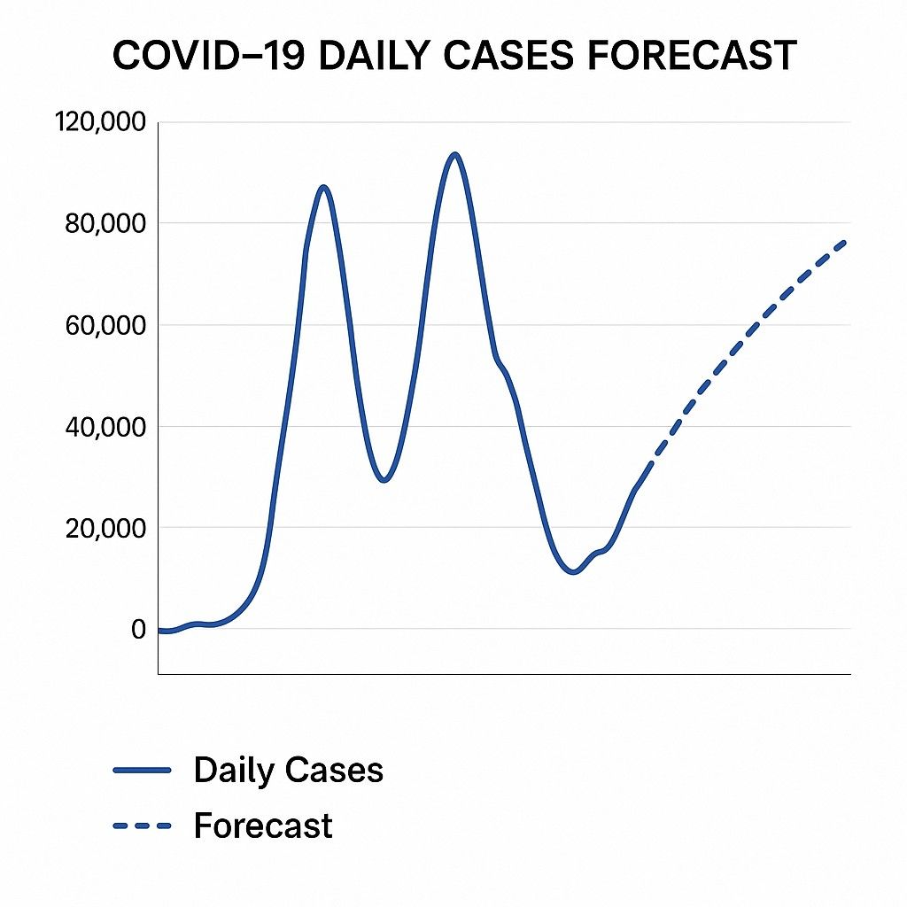
Problem Statement

Accurate prediction of daily COVID-19 cases is essential for health planning, hospital resource allocation, and containment strategies.

Objective

Forecast daily confirmed COVID-19 cases based on historical trends using time series techniques.

Dataset Source

Techniques and Concepts

Rolling averages and smoothing
Curve fitting with Prophet
LSTM for long-term sequential prediction
ARIMA and exponential smoothing

Tools and Libraries

Python, pandas, Prophet, Keras, matplotlib

Expected Outcome

A forecast of daily new cases over the next 7 to 30 days with uncertainty intervals and performance visualizations.

Sample Code Snippet

				
					from prophet import Prophet
import pandas as pd

df = pd.read_csv('covid_data.csv')
df = df[['Date', 'Confirmed']]
df.columns = ['ds', 'y']

model = Prophet()
model.fit(df)

future = model.make_future_dataframe(periods=14)
forecast = model.predict(future)
forecast[['ds', 'yhat', 'yhat_lower', 'yhat_upper']].tail()

Video Tutorial Suggestions

“COVID Case Forecasting with Prophet”
“Time Series for Public Health Analytics”
“Pandemic Forecasting with Deep Learning”

Time Series Project 4 : Retail Sales Forecasting

Problem Statement

Retailers need to accurately predict future sales to optimize inventory, reduce overstock or stockouts, and improve revenue forecasting.

Objective

Develop a model that forecasts future sales at the product or store level using historical data and calendar variables.

Dataset Source

Techniques and Concepts

Time series decomposition
Feature engineering (holiday, store type, promo)
SARIMA and Prophet for time series modeling
XGBoost/LightGBM with temporal data

Tools and Libraries

Python, pandas, Prophet, XGBoost, LightGBM, matplotlib, seaborn

Expected Outcome

A prediction system that estimates store or item sales for the next weeks or months, including holidays and promotions.

Sample Code Snippet

				
					import pandas as pd
from sklearn.ensemble import GradientBoostingRegressor

df = pd.read_csv('sales.csv')
features = ['Store', 'Promo', 'DayOfWeek', 'Month']
target = df['Sales']

model = GradientBoostingRegressor()
model.fit(df[features], target)

future_sales = model.predict(df[features].tail(5))
print(future_sales)

Video Tutorial Suggestions

“Sales Forecasting with Python and Machine Learning”
“Retail Forecasting with XGBoost”
“Time Series + Categorical Features for Store Predictions”

NLP Project Ideas

NLP Project 1 : Twitter Sentiment Analysis

Problem Statement

Brands, marketers, and political analysts need to understand public opinion in real-time to drive decisions, monitor crises, and adjust campaigns accordingly.

Objective

Develop a sentiment analysis model that classifies tweets as positive, negative, or neutral using supervised learning or transformer-based models.

Dataset Sources

Techniques & Concepts

Text preprocessing (cleaning, tokenization, lemmatization)
TF-IDF or word embeddings (Word2Vec, GloVe)
Machine learning (Logistic Regression, Naive Bayes) or deep learning (LSTM, BERT)
Visualization (word clouds, sentiment trends)

Tools & Libraries

Python, NLTK, Scikit-learn, Keras, TensorFlow, Hugging Face Transformers, Tweepy

Expected Outcome

A web or script-based application that takes a tweet or hashtag and returns sentiment classification with accuracy metrics.

Sample Code Snippet

				
					import pandas as pd
from sklearn.feature_extraction.text import TfidfVectorizer
from sklearn.linear_model import LogisticRegression
from sklearn.model_selection import train_test_split

df = pd.read_csv('tweets.csv')
X = df['text']
y = df['sentiment']

vectorizer = TfidfVectorizer(max_features=3000)
X_vect = vectorizer.fit_transform(X)

X_train, X_test, y_train, y_test = train_test_split(X_vect, y, test_size=0.2)
model = LogisticRegression()
model.fit(X_train, y_train)

print(model.score(X_test, y_test))

Video Tutorial Suggestions

Real-Time Twitter Sentiment Dashboard with Python
Sentiment Analysis Using BERT and Hugging Face
Twitter API with Tweepy and Text Classification

NLP Project 2: Resume Parser Using NLP

Problem Statement

Hiring teams need to extract structured information like name, skills, experience, and education from thousands of unstructured resumes quickly and accurately.

Objective

Create an automated parser that uses Named Entity Recognition (NER) and regular expressions to extract key details from resumes in PDF or DOCX formats.

Dataset Sources

Techniques & Concepts

PDF and DOCX parsing
Named Entity Recognition (NER)
Regex-based keyword extraction
Skill matching using dictionaries or embeddings

Tools & Libraries

Python, spaCy, PyPDF2, docx2txt, NLTK, pandas

Expected Outcome

A tool or API that extracts structured resume data and outputs it in JSON or CSV format, ready for ATS integration.

Sample Code Snippet

				
					import docx2txt
import spacy

nlp = spacy.load('en_core_web_sm')
text = docx2txt.process("sample_resume.docx")
doc = nlp(text)

for ent in doc.ents:
    print(ent.text, ent.label_)

Video Tutorial Suggestions

Building a Resume Parser with Python and spaCy
NLP for HR Automation: Resume Screening
Extracting Named Entities from Documents

NLP Project 3: News Article Classification

Problem Statement

News platforms and aggregators need to categorize large volumes of articles into topics like politics, business, and technology to enhance navigation and personalization.

Objective

Train a multi-class text classification model to predict the category of a news article based on its headline and content.

Dataset Sources

Techniques & Concepts

TF-IDF and CountVectorizer
Naive Bayes or Multinomial Logistic Regression
BERT or RoBERTa for advanced contextual classification
Cross-validation and evaluation (F1-score, confusion matrix)

Tools & Libraries

Python, Scikit-learn, Hugging Face Transformers, TensorFlow, pandas

Expected Outcome

A script or application that classifies a new article into categories like world, tech, sports, or health.

Sample Code Snippet

				
					from sklearn.feature_extraction.text import TfidfVectorizer
from sklearn.naive_bayes import MultinomialNB
from sklearn.model_selection import train_test_split

df = pd.read_csv('news.csv')
X = df['text']
y = df['category']

vectorizer = TfidfVectorizer(max_features=5000)
X_vect = vectorizer.fit_transform(X)

X_train, X_test, y_train, y_test = train_test_split(X_vect, y, test_size=0.2)
model = MultinomialNB()
model.fit(X_train, y_train)

print(model.score(X_test, y_test))

Video Tutorial Suggestions

News Article Classifier Using Python and TF-IDF
BERT Fine-Tuning for Text Classification
End-to-End NLP Project: News Categorization

NLP Project 4: Text Summarization with Transformers

Problem Statement

Professionals need to read lengthy documents, news articles, or reports. Automated summarization can save hours and improve productivity.

Objective

Build a text summarization model that generates concise summaries of longer texts using extractive or abstractive techniques.

Dataset Sources

Techniques & Concepts

Extractive methods (TextRank, LexRank)
Abstractive summarization with transformers (BART, T5, Pegasus)
Tokenization and input chunking
ROUGE scoring for summary evaluation

Tools & Libraries

Python, Hugging Face Transformers, TensorFlow, spaCy, NLTK

Expected Outcome

A functional summarizer that reduces long-form articles into readable 3–5 sentence summaries suitable for newsletters, dashboards, or reports.

Sample Code Snippet

				
					from transformers import pipeline

summarizer = pipeline("summarization", model="facebook/bart-large-cnn")
text = """Artificial Intelligence is transforming multiple industries across the globe..."""
summary = summarizer(text, max_length=120, min_length=30, do_sample=False)

print(summary[0]['summary_text'])

Video Tutorial Suggestions

Abstractive Summarization with Transformers
Text Summarization Using BART and Hugging Face
Building Your Own Summarizer with T5

Recommendation System Projects

1. Book Recommendation System

Problem Statement

With thousands of books available online, users often struggle to find titles tailored to their interests or preferences.

Objective

Build a content-based and/or collaborative filtering book recommendation engine that suggests books based on user ratings or book metadata.

Dataset Source

Techniques & Concepts

User-Item Matrix
Cosine Similarity for content-based filtering
KNN or Matrix Factorization (SVD, ALS)
TF-IDF for metadata matching (genre, description, author)

Tools & Libraries

Python, Scikit-learn, Pandas, Surprise, Streamlit (optional)

Expected Outcome

An interactive system that allows users to input a book and receive top-N similar recommendations based on their taste or item profile.

Sample Code Snippet

				
					from sklearn.feature_extraction.text import TfidfVectorizer
from sklearn.metrics.pairwise import cosine_similarity
import pandas as pd

# Load dataset
df = pd.read_csv('books.csv')
tfidf = TfidfVectorizer(stop_words='english')
tfidf_matrix = tfidf.fit_transform(df['Book-Title'])

# Compute similarity
cosine_sim = cosine_similarity(tfidf_matrix, tfidf_matrix)

def recommend_books(title, cosine_sim=cosine_sim):
    idx = df[df['Book-Title'] == title].index[0]
    sim_scores = list(enumerate(cosine_sim[idx]))
    sim_scores = sorted(sim_scores, key=lambda x: x[1], reverse=True)[1:6]
    book_indices = [i[0] for i in sim_scores]
    return df['Book-Title'].iloc[book_indices]

print(recommend_books("The Hobbit"))

Video Tutorial Suggestions

“Book Recommendation Engine using Python and Pandas”
“Build a Content-Based Recommender System in 30 Minutes”
“Collaborative Filtering vs Content-Based Filtering Explained”

2. Product Suggestion Model (E-commerce)

Problem Statement

E-commerce platforms like Amazon need scalable product recommendation systems to personalize user experience and increase sales.

Objective

Build a product recommendation engine that suggests similar or complementary items based on user purchase history or item similarity.

Dataset Source

Techniques & Concepts

Collaborative filtering (User-User and Item-Item)
Market basket analysis (Apriori or FP-Growth)
ALS matrix factorization (Spark MLlib)
Content-based recommendations using metadata

Tools & Libraries

Python, Surprise, LightFM, PySpark, Scikit-learn

Expected Outcome

A model that suggests frequently bought together items, similar products, or cross-sell/up-sell combos based on user interaction data.

Sample Code Snippet

				
					from surprise import Dataset, Reader, SVD
from surprise.model_selection import train_test_split

# Load dataset
data = Dataset.load_builtin('ml-100k')  # or custom dataset
trainset, testset = train_test_split(data, test_size=0.2)

# Train SVD model
model = SVD()
model.fit(trainset)

# Predict
pred = model.predict(uid='196', iid='242')
print(f"Predicted Rating: {pred.est}")

Video Tutorial Suggestions

“E-commerce Recommender System using SVD”
“Amazon Style Recommendation System with LightFM”
“Collaborative Filtering with Surprise Library”

3. Music Recommendation Engine

Problem Statement

Music platforms like Spotify and YouTube Music need intelligent systems to suggest songs based on listener behavior, mood, or audio features.

Objective

Create a personalized music recommender using song metadata, audio features, or listening patterns.

Dataset Source

Techniques & Concepts

Content-based filtering using audio features (tempo, valence, energy)
K-means clustering for genre/mood segmentation
Matrix factorization for collaborative filtering
Deep learning (autoencoders for embeddings)

Tools & Libraries

Python, Scikit-learn, Spotipy (Spotify API), TensorFlow, Keras

Expected Outcome

A model that recommends similar tracks based on tempo, mood, genre, or listener similarity.

Sample Code Snippet

				
					from sklearn.preprocessing import StandardScaler
from sklearn.neighbors import NearestNeighbors
import pandas as pd

df = pd.read_csv('spotify.csv')
features = ['danceability', 'energy', 'tempo', 'valence']
X = StandardScaler().fit_transform(df[features])

model = NearestNeighbors(n_neighbors=6, algorithm='ball_tree')
model.fit(X)

def recommend_song(index):
    distances, indices = model.kneighbors([X[index]])
    return df.iloc[indices[0]]['track_name']

print(recommend_song(10))

Video Tutorial Suggestions

“Spotify Song Recommender with Python”
“Music Clustering using K-Means”
“Build a Music Recommendation Engine from Audio Features”

4. News Article Recommender

Problem Statement

News websites want to improve user engagement by suggesting relevant articles based on past reading behavior and content interest.

Objective

Build a news recommender that serves relevant content using NLP techniques and user browsing history.

Dataset Source

MIND News Dataset (Microsoft)
AG News Dataset (Kaggle)

Techniques & Concepts

NLP-based content similarity using TF-IDF or BERT embeddings
Real-time clickstream-based collaborative filtering
News topic clustering and personalization
Multi-armed bandit (optional) for reinforcement

Tools & Libraries

Python, Scikit-learn, Hugging Face Transformers (for BERT), Faiss, FastAPI

Expected Outcome

A system that recommends news articles similar in topic or tone to a user’s reading preferences or clicked articles.

Sample Code Snippet

				
					from sklearn.feature_extraction.text import TfidfVectorizer
from sklearn.metrics.pairwise import linear_kernel
import pandas as pd

df = pd.read_csv('news_data.csv')
tfidf = TfidfVectorizer(stop_words='english')
tfidf_matrix = tfidf.fit_transform(df['title'] + ' ' + df['content'])

cos_sim = linear_kernel(tfidf_matrix, tfidf_matrix)

def recommend_news(title, cosine_sim=cos_sim):
    idx = df[df['title'] == title].index[0]
    sim_scores = list(enumerate(cosine_sim[idx]))
    sim_scores = sorted(sim_scores, key=lambda x: x[1], reverse=True)[1:6]
    indices = [i[0] for i in sim_scores]
    return df['title'].iloc[indices]

print(recommend_news("India launches new satellite"))

Video Tutorial Suggestions

“Build a News Recommender System with NLP”
“Content-Based News Article Recommender with BERT”
“Hybrid News Recommendation System in Python”

Computer Vision Project Ideas

1. Face Mask Detection (Real-Time Compliance Monitor)

Problem Statement

In public spaces and hospitals, ensuring that people wear face masks is essential for public safety. Manual monitoring is inefficient.

Objective

Build a real-time face mask detection system using deep learning and OpenCV to detect whether a person is wearing a mask or not.

Dataset Source

Techniques & Concepts

CNN for image classification
Real-time video feed detection
Face detection (Haar cascades, Dlib, MTCNN)
MobileNetV2 transfer learning

Tools & Libraries

Python, TensorFlow/Keras, OpenCV, NumPy, Streamlit (for demo)

Expected Outcome

A live camera app that detects faces and classifies them into “Mask” or “No Mask” in real time.

Sample Code Snippet

				
					import cv2
from keras.models import load_model
import numpy as np

# Load model
model = load_model('mask_detector_model.h5')

# Load video
cap = cv2.VideoCapture(0)

while True:
    ret, frame = cap.read()
    face = cv2.resize(frame, (224, 224)) / 255.0
    prediction = model.predict(np.expand_dims(face, axis=0))[0]

    label = "Mask" if prediction[0] > 0.5 else "No Mask"
    cv2.putText(frame, label, (20, 50), cv2.FONT_HERSHEY_SIMPLEX, 1, (255, 0, 0), 2)
    cv2.imshow('Face Mask Detector', frame)
    
    if cv2.waitKey(1) & 0xFF == ord('q'):
        break
cap.release()
cv2.destroyAllWindows()

Video Tutorial Suggestions

“Real-Time Face Mask Detection with OpenCV & Python”
“How to Build a COVID Mask Detection App”
“Deploying Face Mask Detection with Streamlit”

2. Road Lane Line Detection (Self-Driving Cars)

Problem Statement

Lane detection is crucial for autonomous driving systems to maintain vehicle trajectory and safety.

Objective

Build a computer vision pipeline that detects road lanes from dashcam videos in real time.

Dataset Source

Techniques & Concepts

Canny edge detection
Region of interest (ROI) masking
Hough Line Transform
Frame-by-frame lane overlay

Tools & Libraries

Python, OpenCV, NumPy, Matplotlib

Expected Outcome

A video or dashboard showing lane overlays in real-time or recorded driving footage.

Sample Code Snippet

				
					import cv2
import numpy as np

def region_of_interest(image):
    height = image.shape[0]
    polygons = np.array([[(0, height), (image.shape[1], height), (500, 250)]])
    mask = np.zeros_like(image)
    cv2.fillPoly(mask, polygons, 255)
    return cv2.bitwise_and(image, mask)

def detect_lanes(frame):
    gray = cv2.cvtColor(frame, cv2.COLOR_BGR2GRAY)
    edges = cv2.Canny(gray, 50, 150)
    cropped = region_of_interest(edges)
    lines = cv2.HoughLinesP(cropped, 2, np.pi / 180, 100, np.array([]), minLineLength=40, maxLineGap=5)
    if lines is not None:
        for line in lines:
            x1, y1, x2, y2 = line[0]
            cv2.line(frame, (x1, y1), (x2, y2), (0, 255, 0), 5)
    return frame

Video Tutorial Suggestions

“Road Lane Detection for Self-Driving Cars”
“Computer Vision Project: Detect Lanes with OpenCV”
“Building Autonomous Navigation System in Python”

3. Pneumonia Detection from Chest X-rays

Problem Statement

Detecting pneumonia from X-ray images is time-consuming and requires experienced radiologists. AI can help automate early diagnosis.

Objective

Train a CNN model to classify X-ray images into “Pneumonia” and “Normal” using transfer learning.

Dataset Source

Chest X-ray Pneumonia Dataset (Kaggle)

Techniques & Concepts

Image classification
Transfer learning with ResNet or VGG
Image augmentation
Evaluation: accuracy, AUC, recall

Tools & Libraries

Python, Keras/TensorFlow, Matplotlib, OpenCV

Expected Outcome

A classification model that identifies pneumonia in X-ray images with high accuracy and can be deployed in medical screening apps.

Sample Code Snippet

				
					from tensorflow.keras.applications import VGG16
from tensorflow.keras.preprocessing.image import ImageDataGenerator
from tensorflow.keras import layers, models

# Load VGG16 base
base_model = VGG16(include_top=False, input_shape=(224, 224, 3), weights='imagenet')
model = models.Sequential([
    base_model,
    layers.Flatten(),
    layers.Dense(128, activation='relu'),
    layers.Dense(1, activation='sigmoid')
])
model.compile(optimizer='adam', loss='binary_crossentropy', metrics=['accuracy'])

# Load dataset
train_gen = ImageDataGenerator(rescale=1./255).flow_from_directory('chest_xray/train', target_size=(224, 224))
model.fit(train_gen, epochs=5)

Video Tutorial Suggestions

“Pneumonia Detection from Chest X-Rays using CNN”
“AI in Medical Imaging: Pneumonia Classifier”
“Transfer Learning for Radiology with VGG16”

4. Real-Time Face Emotion Recognition

Problem Statement

Emotion recognition is critical for applications in e-learning, mental health monitoring, and human-computer interaction.

Objective

Detect and classify human emotions from facial expressions in real-time video feeds.

Dataset Source

Techniques & Concepts

CNN for facial expression recognition
Real-time face detection using Haar cascades
Multiclass classification (Happy, Sad, Angry, etc.)
Data augmentation for expression generalization

Tools & Libraries

Python, TensorFlow/Keras, OpenCV, Dlib, Matplotlib

Expected Outcome

A web camera-based application that labels emotional states (e.g., happy, angry, sad) with accuracy and real-time feedback.

Sample Code Snippet

				
					import cv2
from keras.models import load_model
import numpy as np

emotion_model = load_model('emotion_model.h5')
emotion_labels = ['Angry', 'Disgust', 'Fear', 'Happy', 'Neutral', 'Sad', 'Surprise']

cap = cv2.VideoCapture(0)
face_detector = cv2.CascadeClassifier(cv2.data.haarcascades + 'haarcascade_frontalface_default.xml')

while True:
    _, frame = cap.read()
    gray = cv2.cvtColor(frame, cv2.COLOR_BGR2GRAY)
    faces = face_detector.detectMultiScale(gray, 1.3, 5)
    for (x, y, w, h) in faces:
        roi = gray[y:y+h, x:x+w]
        roi = cv2.resize(roi, (48, 48)) / 255.0
        roi = roi.reshape(1, 48, 48, 1)
        prediction = emotion_model.predict(roi)
        label = emotion_labels[np.argmax(prediction)]
        cv2.putText(frame, label, (x, y-10), cv2.FONT_HERSHEY_SIMPLEX, 0.9, (255, 0, 255), 2)
        cv2.rectangle(frame, (x, y), (x+w, y+h), (255, 0, 0), 2)
    cv2.imshow("Emotion Recognition", frame)
    if cv2.waitKey(1) & 0xFF == ord('q'):
        break
cap.release()
cv2.destroyAllWindows()

Video Tutorial Suggestions

“Real-Time Emotion Detection with CNN and OpenCV”
“Facial Expression Recognition with FER2013”
“Build Emotion AI with Python Step-by-Step”

Real-World Industry-Focused Projects

Healthcare Data Science Projects

1. Patient Risk Scoring System

Problem Statement

Hospitals need to identify high-risk patients early to prevent readmissions, improve outcomes, and allocate ICU resources efficiently.

Objective

Build a patient risk scoring system to classify patients into high, medium, or low-risk categories based on vitals, lab results, and medical history.

Dataset Source

MIMIC-III or MIMIC-IV (MIT PhysioNet)
Heart Disease UCI Dataset

Techniques & Concepts

Classification (Logistic Regression, XGBoost, SVM)
Feature importance using SHAP values
Risk bucket segmentation
ROC-AUC, recall, and precision evaluation

Tools & Libraries

Python, Scikit-learn, SHAP, Pandas, Seaborn, Streamlit

Expected Outcome

A system that outputs a risk score for patients and flags high-risk individuals for proactive intervention.

Sample Code Snippet

				
					import pandas as pd
from sklearn.ensemble import GradientBoostingClassifier
from sklearn.metrics import classification_report
from sklearn.model_selection import train_test_split

# Load data
df = pd.read_csv('patient_data.csv')

# Feature engineering
X = df.drop('high_risk', axis=1)
y = df['high_risk']  # 1 = high-risk, 0 = others

# Train-test split
X_train, X_test, y_train, y_test = train_test_split(X, y, test_size=0.2)

# Model
model = GradientBoostingClassifier()
model.fit(X_train, y_train)

# Predict
y_pred = model.predict(X_test)
print(classification_report(y_test, y_pred))

Video Tutorial Suggestions

“Building a Risk Prediction Model in Healthcare with Python”
“Patient Monitoring System with Machine Learning”
“SHAP for Interpreting Medical Risk Models”

2. Disease Diagnosis Using Symptoms

Problem Statement

General practitioners often receive vague symptoms, making early disease identification difficult without clinical tests.

Objective

Use machine learning to predict possible diseases based on symptom inputs provided by patients or wearable devices.

Dataset Source

Techniques & Concepts

Multi-class classification (Naive Bayes, Random Forest, Neural Nets)
Text vectorization of symptoms (TF-IDF, One-hot encoding)
Symptom clustering
Evaluation via confusion matrix, precision, and recall

Tools & Libraries

Python, Pandas, Scikit-learn, NLTK, Streamlit

Expected Outcome

A model that provides a top-k ranked list of likely diseases based on user-entered symptoms, useful for triage and preliminary diagnosis.

Sample Code Snippet

				
					import pandas as pd
from sklearn.naive_bayes import MultinomialNB
from sklearn.feature_extraction.text import CountVectorizer
from sklearn.model_selection import train_test_split

# Load dataset
df = pd.read_csv('disease_symptoms.csv')

# Vectorize symptoms
vectorizer = CountVectorizer()
X = vectorizer.fit_transform(df['symptoms'])
y = df['disease']

# Train-test split
X_train, X_test, y_train, y_test = train_test_split(X, y, test_size=0.2)

# Model
model = MultinomialNB()
model.fit(X_train, y_train)

# Predict
y_pred = model.predict(X_test)
print("Sample Prediction:", y_pred[:5])

Video Tutorial Suggestions

“AI Symptom Checker with Python”
“Medical Diagnosis from Text Input Using NLP”
“Build a Disease Prediction Model with Machine Learning”

3. Medical Image Segmentation (Tumor/Organ Detection)

Problem Statement

Manual image annotation by radiologists is time-consuming and prone to subjective interpretation. Accurate segmentation is critical for diagnostics and surgery planning.

Objective

Use deep learning to segment medical images and highlight areas of concern such as tumors, lungs, or other organs.

Dataset Source

Brain Tumor MRI Dataset
LUNA16 CT Scans
ISIC Skin Lesion Segmentation Dataset

Techniques & Concepts

Convolutional Neural Networks (CNNs)
U-Net, SegNet, or DeepLabV3+ architecture
Dice coefficient, IoU (Intersection over Union)
Preprocessing: resizing, normalization, augmentation

Tools & Libraries

Python, TensorFlow/Keras or PyTorch, OpenCV, NumPy, Matplotlib

Expected Outcome

A fully trained model that segments critical regions in MRI, CT, or dermoscopic images and can be integrated into a clinical pipeline.

Sample Code Snippet (U-Net in Keras)

				
					from tensorflow.keras.models import Model
from tensorflow.keras.layers import Input, Conv2D, MaxPooling2D, UpSampling2D, concatenate

def unet(input_size=(128, 128, 1)):
    inputs = Input(input_size)
    c1 = Conv2D(64, 3, activation='relu', padding='same')(inputs)
    p1 = MaxPooling2D()(c1)
    c2 = Conv2D(128, 3, activation='relu', padding='same')(p1)
    u1 = UpSampling2D()(c2)
    merge = concatenate([u1, c1])
    c3 = Conv2D(64, 3, activation='relu', padding='same')(merge)
    outputs = Conv2D(1, 1, activation='sigmoid')(c3)
    model = Model(inputs, outputs)
    model.compile(optimizer='adam', loss='binary_crossentropy', metrics=['accuracy'])
    return model

Video Tutorial Suggestions

“Medical Image Segmentation with U-Net in Python”
“Brain Tumor Detection Using CNNs and MRI Images”
“Deep Learning for Radiology Image Processing”

Financial Data Science Projects

1. Loan Approval Prediction

Problem Statement

Banks and NBFCs face high operational costs and default risks due to inaccurate or manual loan approval processes.

Objective

Build a machine learning model to predict whether a loan application should be approved based on applicant profile, income, credit history, and other factors.

Dataset Source

Loan Prediction Dataset (Analytics Vidhya)
Lending Club open dataset
Simulated bank loan application data

Techniques & Concepts

Binary classification
Feature encoding (categorical → numerical)
Handling missing values
Evaluation with ROC-AUC, confusion matrix

Tools & Libraries

Python, Pandas, Scikit-learn, XGBoost, Matplotlib

Expected Outcome

A predictive model that helps automate loan approvals, reducing processing time and improving accuracy.

Sample Code Snippet

				
					import pandas as pd
from sklearn.model_selection import train_test_split
from sklearn.ensemble import RandomForestClassifier
from sklearn.metrics import classification_report

# Load data
df = pd.read_csv('loan_data.csv')

# Preprocessing
df.fillna(method='ffill', inplace=True)
df = pd.get_dummies(df, drop_first=True)

# Features and target
X = df.drop('Loan_Status', axis=1)
y = df['Loan_Status'].map({'Y': 1, 'N': 0})

# Split and train
X_train, X_test, y_train, y_test = train_test_split(X, y, test_size=0.2)
model = RandomForestClassifier()
model.fit(X_train, y_train)

# Predict
y_pred = model.predict(X_test)
print(classification_report(y_test, y_pred))

Video Tutorial Suggestions

“Loan Approval Prediction Project with Scikit-learn”
“End-to-End Loan Classification with Python”
“Banking ML Models for Beginners”

2. Credit Risk Scoring Model

Problem Statement

Accurately evaluating a customer’s creditworthiness is essential to reduce defaults and non-performing assets (NPAs).

Objective

Build a model that scores customer risk into low, medium, or high credit risk tiers using demographic, financial, and behavioral features.

Dataset Source

German Credit Risk Dataset (UCI)
LendingClub loan book
Credit bureau-simulated datasets

Techniques & Concepts

Multi-class classification
Feature importance analysis
Weight of Evidence (WoE) and Information Value (IV)
Confusion matrix and ROC analysis

Tools & Libraries

Python, Pandas, Scikit-learn, XGBoost, SHAP, Streamlit (optional for deployment)

Expected Outcome

A credit scoring system that ranks borrowers and informs risk-based interest rates or credit limits.

Sample Code Snippet

				
					import pandas as pd
from sklearn.ensemble import GradientBoostingClassifier
from sklearn.metrics import classification_report
from sklearn.model_selection import train_test_split

# Load data
df = pd.read_csv('credit_risk_data.csv')

# Feature prep
X = df.drop('Risk', axis=1)
y = df['Risk']  # Low, Medium, High

# Encode and split
X = pd.get_dummies(X, drop_first=True)
X_train, X_test, y_train, y_test = train_test_split(X, y, test_size=0.2)

# Train model
model = GradientBoostingClassifier()
model.fit(X_train, y_train)

# Evaluate
y_pred = model.predict(X_test)
print(classification_report(y_test, y_pred))

Video Tutorial Suggestions

“Credit Risk Scoring with Python and German Dataset”
“How to Use WoE and IV in Credit Models”
“ML for FinTech: Build Your Own Credit Scorecard”

3. Stock Portfolio Optimization

Problem Statement

Retail and institutional investors often rely on intuition rather than data to build investment portfolios, leading to suboptimal returns.

Objective

Use modern portfolio theory and machine learning to create an optimized stock portfolio with maximum returns for a given level of risk.

Dataset Source

Techniques & Concepts

Mean-variance optimization (Markowitz Theory)
Sharpe Ratio and risk-return tradeoff
Monte Carlo simulation
Correlation matrix and diversification strategy

Tools & Libraries

Python, NumPy, Pandas, yfinance, Matplotlib, cvxpy or PyPortfolioOpt

Expected Outcome

An optimized portfolio of stocks with calculated weights, expected returns, and risk levels, ideal for algorithmic investing or Robo-advisors.

Sample Code Snippet

				
					import yfinance as yf
import numpy as np
import pandas as pd
import matplotlib.pyplot as plt

# Load historical data
tickers = ['AAPL', 'MSFT', 'GOOGL', 'AMZN']
data = yf.download(tickers, start='2022-01-01', end='2023-01-01')['Adj Close']

# Calculate daily returns and mean
returns = data.pct_change().dropna()
mean_returns = returns.mean()
cov_matrix = returns.cov()

# Portfolio weights (equal for now)
weights = np.array([0.25, 0.25, 0.25, 0.25])
port_return = np.dot(weights, mean_returns) * 252
port_risk = np.sqrt(np.dot(weights.T, np.dot(cov_matrix * 252, weights)))

print(f"Annual Expected Return: {port_return:.2f}")
print(f"Annual Portfolio Risk (Std Dev): {port_risk:.2f}")

Video Tutorial Suggestions

“Stock Portfolio Optimization with Python”
“Markowitz Theory Explained for Data Scientists”
“Build Your Own Robo-Advisor Using PyPortfolioOpt”

E-commerce Projects

1. Customer Lifetime Value (CLV) Prediction

Problem Statement

Customer acquisition is expensive. To maximize ROI, businesses must identify customers with high long-term value and target them with retention-focused strategies.

Objective

Build a regression or probabilistic model to predict Customer Lifetime Value (CLV) using transactional, behavioral, and demographic data.

Dataset Source

Techniques & Concepts

RFM analysis (Recency, Frequency, Monetary)
Linear Regression, XGBoost, or Gamma-Gamma model
LTV segmentation for marketing campaigns
CLTV scoring and visualization

Tools & Libraries

Python, Lifetimes (for probabilistic modeling), Pandas, Scikit-learn, Matplotlib, Plotly

Expected Outcome

A model that segments customers by predicted LTV (High, Medium, Low) to support retention, reactivation, and upselling strategies.

Sample Code Snippet

				
					from lifetimes import BetaGeoFitter, GammaGammaFitter
import pandas as pd

# Load and prepare data
df = pd.read_csv('online_retail.csv')
summary = summary_data_from_transaction_data(df, 'CustomerID', 'InvoiceDate', monetary_value_col='TotalAmount')

# Fit BG/NBD model
bgf = BetaGeoFitter()
bgf.fit(summary['frequency'], summary['recency'], summary['T'])

# Fit Gamma-Gamma model
ggf = GammaGammaFitter()
ggf.fit(summary['frequency'], summary['monetary_value'])

# Predict CLV for 6 months
summary['clv'] = ggf.customer_lifetime_value(
    bgf, summary['frequency'], summary['recency'], summary['T'],
    summary['monetary_value'], time=6, freq='D'
)

Video Tutorial Suggestions

“Predicting Customer Lifetime Value in Python”
“CLTV Modeling for Subscription and Retail Businesses”
“RFM and LTV Analysis with Real Data”

2. Product Sentiment Analysis (Customer Reviews NLP Project)

Problem Statement

E-commerce platforms receive thousands of product reviews daily. Manually processing these for insight is not scalable or consistent.

Objective

Use Natural Language Processing to classify product reviews into positive, neutral, or negative sentiment categories, helping improve product development and customer service.

Dataset Source

Amazon Product Review Dataset
Flipkart or eBay review datasets (scraped or simulated)

Techniques & Concepts

Text preprocessing and vectorization (TF-IDF, Word2Vec)
Sentiment classification using Logistic Regression or BERT
Word clouds and keyphrase extraction
Multiclass classification and F1-score evaluation

Tools & Libraries

Python, NLTK, Scikit-learn, SpaCy, TensorFlow/Keras (for BERT), Seaborn

Expected Outcome

A sentiment analysis model that provides brand insights from customer feedback and helps in product ratings prediction.

Sample Code Snippet

				
					from sklearn.feature_extraction.text import TfidfVectorizer
from sklearn.linear_model import LogisticRegression
from sklearn.model_selection import train_test_split
from sklearn.metrics import classification_report
import pandas as pd

# Load data
df = pd.read_csv('product_reviews.csv')
X = df['review_text']
y = df['sentiment']  # positive, neutral, negative

# TF-IDF vectorization
tfidf = TfidfVectorizer(max_features=5000)
X_tfidf = tfidf.fit_transform(X)

# Train-test split
X_train, X_test, y_train, y_test = train_test_split(X_tfidf, y, test_size=0.2)

# Train model
model = LogisticRegression()
model.fit(X_train, y_train)

# Evaluate
y_pred = model.predict(X_test)
print(classification_report(y_test, y_pred))

Video Tutorial Suggestions

“Product Review Sentiment Analysis with Scikit-learn”
“NLP Project: Classify Amazon Reviews”
“Fine-tuning BERT for Sentiment Classification”

3. Shopping Cart Abandonment Predictor

Problem Statement

A large percentage of users add items to their cart but never complete the purchase. Identifying the behavioral patterns behind this can significantly boost conversions.

Objective

Build a binary classification model that predicts if a customer will abandon their cart before purchase, based on session behavior, time spent, clicks, and items viewed.

Dataset Source

Techniques & Concepts

Binary classification (Logistic Regression, Random Forest)
Session-based features and clickstream analysis
Class imbalance handling (SMOTE, threshold tuning)
Behavioral funnel visualization

Tools & Libraries

Python, Pandas, Scikit-learn, XGBoost, Matplotlib, Streamlit (for demo app)

Expected Outcome

A real-time predictor for abandonment that can trigger retargeting actions like email reminders, discount offers, or chatbot prompts.

Sample Code Snippet

				
					from sklearn.ensemble import RandomForestClassifier
from sklearn.model_selection import train_test_split
from sklearn.metrics import accuracy_score
import pandas as pd

# Load session data
df = pd.read_csv('shopping_cart_data.csv')

# Features and label
X = df[['pages_viewed', 'time_on_site', 'cart_items', 'previous_purchases']]
y = df['abandoned']  # 0 = completed, 1 = abandoned

# Train-test split
X_train, X_test, y_train, y_test = train_test_split(X, y, test_size=0.2)

# Train model
model = RandomForestClassifier()
model.fit(X_train, y_train)

# Evaluate
y_pred = model.predict(X_test)
print(f"Accuracy: {accuracy_score(y_test, y_pred)}")

Video Tutorial Suggestions

“Predict Shopping Cart Abandonment Using Machine Learning”
“Customer Behavior Prediction with Clickstream Data”
“E-Commerce Funnel Analysis with Python and Streamlit”

HR & Employee Analytics

1. Employee Attrition Prediction (Churn Analysis)

Problem Statement

Employee turnover is costly and disrupts team productivity. HR teams struggle to predict which employees are at risk of leaving and why.

Objective

Build a machine learning model to predict whether an employee is likely to leave the organization, based on factors like job role, satisfaction, salary, and tenure.

Dataset Source

IBM HR Analytics Employee Attrition Dataset

Techniques & Concepts

Binary classification
Feature importance analysis (e.g., SHAP)
Handling class imbalance (SMOTE, class weights)
HR dashboard metrics (voluntary vs involuntary attrition)

Tools & Libraries

Python, Pandas, Scikit-learn, XGBoost, SHAP, Streamlit for deployment

Expected Outcome

A predictive model and dashboard to alert HR teams about employees at high risk of attrition and suggest intervention strategies.

Sample Code Snippet

				
					import pandas as pd
from sklearn.ensemble import RandomForestClassifier
from sklearn.model_selection import train_test_split
from sklearn.metrics import classification_report
from imblearn.over_sampling import SMOTE

# Load dataset
df = pd.read_csv('employee_attrition.csv')

# Features and label
X = df.drop('Attrition', axis=1)
y = df['Attrition'].map({'Yes': 1, 'No': 0})

# Handle imbalance
sm = SMOTE()
X_res, y_res = sm.fit_resample(X, y)

# Train-test split
X_train, X_test, y_train, y_test = train_test_split(X_res, y_res, test_size=0.2)

# Train model
model = RandomForestClassifier()
model.fit(X_train, y_train)

# Predict
y_pred = model.predict(X_test)
print(classification_report(y_test, y_pred))

Video Tutorial Suggestions

“HR Analytics Project: Predicting Employee Attrition”
“How to Handle Class Imbalance in HR Datasets”
“Deploying Employee Churn Model with Streamlit”

2. Resume Matching Algorithm for Automated Recruitment

Problem Statement

Recruiters spend hours screening resumes. Manual matching is inefficient and prone to bias, especially when hiring at scale.

Objective

Build a Natural Language Processing (NLP) based system to rank and match candidate resumes with job descriptions based on skill similarity.

Dataset Source

Simulated or scraped job descriptions and resumes
Resume Dataset (Text classification)

Techniques & Concepts

Text preprocessing (tokenization, stopword removal)
TF-IDF and cosine similarity for matching
Named Entity Recognition (skills, tools, degrees)
Ranking system for top candidates

Tools & Libraries

Python, NLTK, SpaCy, Scikit-learn, Gensim, Flask or Streamlit

Expected Outcome

A matching system that takes a job description and ranks uploaded resumes by relevance, speeding up hiring processes.

Sample Code Snippet

				
					from sklearn.feature_extraction.text import TfidfVectorizer
from sklearn.metrics.pairwise import cosine_similarity

# Load resumes and job description
resumes = ["Python developer with ML experience", "Java fullstack engineer", "Data analyst with SQL skills"]
job_desc = "Looking for a data analyst with Python and SQL experience"

# Combine
documents = [job_desc] + resumes

# Vectorize
tfidf = TfidfVectorizer()
tfidf_matrix = tfidf.fit_transform(documents)

# Compute similarity
similarity_scores = cosine_similarity(tfidf_matrix[0:1], tfidf_matrix[1:])
for idx, score in enumerate(similarity_scores[0]):
    print(f'Resume {idx+1} Match Score: {score:.2f}')

Video Tutorial Suggestions

“Resume Screening with NLP and Cosine Similarity”
“AI-Powered Job Matching System with Python”
“Building Resume Parser and Recommender in Streamlit”

3. Workforce Diversity Analytics

Problem Statement

Organizations aim to improve diversity and inclusion, but they often lack data-driven insights into representation, bias, or inequality in hiring and promotion.

Objective

Analyze diversity across gender, ethnicity, department, and experience levels. Identify patterns of inequality and suggest interventions for improvement.

Dataset Source

Simulated HRIS datasets
HR Diversity Dataset on Kaggle

Techniques & Concepts

Descriptive analytics and EDA
Cross-tabulation and group analysis (e.g., by gender/role)
Pay gap analysis
Data storytelling for HR insights

Tools & Libraries

Python, Pandas, Seaborn, Plotly, Tableau or Power BI

Expected Outcome

Interactive dashboards and reports showing diversity stats and recommendations, supporting HR and DEI (Diversity, Equity, Inclusion) initiatives.

Sample Code Snippet

				
					import pandas as pd
import seaborn as sns
import matplotlib.pyplot as plt

# Load dataset
df = pd.read_csv('workforce_diversity.csv')

# Gender distribution by department
dept_gender = df.groupby(['Department', 'Gender']).size().unstack().fillna(0)
dept_gender.plot(kind='bar', stacked=True)
plt.title('Gender Distribution by Department')
plt.ylabel('Count')
plt.xticks(rotation=45)
plt.tight_layout()
plt.show()

Video Tutorial Suggestions

“Analyzing Workforce Diversity with Python”
“Creating HR Dashboards with Plotly and Seaborn”
“Gender Pay Gap Analytics for HR Teams”

Marketing Analytics Data Science Projects

1. Email Campaign Effectiveness Analysis

Problem Statement

Marketers send thousands of promotional emails, but without proper analysis, it’s hard to measure what’s working and what isn’t. Bounce rates, open rates, and conversions can vary drastically across campaigns.

Objective

Build a model to evaluate the effectiveness of email marketing campaigns using KPIs like open rate, click-through rate (CTR), and conversion rate.

Dataset Source

Email Campaign Dataset on Kaggle
Simulated CRM/email log data from Mailchimp or HubSpot exports

Techniques & Concepts

Exploratory data analysis (EDA)
Segmentation by user behavior (opens, clicks)
KPI calculation and visualization
Conversion analysis using funnels and attribution

Tools & Libraries

Python, Pandas, Matplotlib, Seaborn, Tableau or Power BI (optional for dashboards)

Expected Outcome

An analytical report or dashboard showing which campaign performed best and why, with insights to improve future email strategy.

Sample Code Snippet

				
					import pandas as pd
import matplotlib.pyplot as plt

# Load email campaign data
df = pd.read_csv('email_campaign_data.csv')

# Calculate KPIs
df['open_rate'] = df['emails_opened'] / df['emails_sent']
df['ctr'] = df['emails_clicked'] / df['emails_opened']
df['conversion_rate'] = df['conversions'] / df['emails_clicked']

# Visualize campaign performance
df[['campaign_name', 'open_rate', 'ctr', 'conversion_rate']].set_index('campaign_name').plot(kind='bar')
plt.title('Email Campaign Performance Comparison')
plt.ylabel('Rate')
plt.xticks(rotation=45)
plt.tight_layout()
plt.show()

Video Tutorial Suggestions

“Marketing Analytics with Python: Email Campaign Case Study”
“How to Analyze Open Rate and CTR in Pandas”
“Building a Marketing KPI Dashboard in Power BI”

2. A/B Testing Simulator for Marketing Experiments

Problem Statement

Marketers need to test variations of landing pages, headlines, or CTAs. Without statistically valid A/B testing, decisions may be based on intuition rather than data.

Objective

Simulate and evaluate A/B tests using conversion data to understand which variation performs better, using hypothesis testing and confidence intervals.

Dataset Source

Simulated web traffic or email performance datasets
A/B Testing Example Dataset on Kaggle

Techniques & Concepts

Hypothesis testing (Z-test, T-test)
Confidence interval calculation
Power and sample size analysis
Visualization of experiment results

Tools & Libraries

Python, Scipy, Statsmodels, Pandas, Matplotlib

Expected Outcome

A simulator tool or notebook that accepts input metrics (conversions, traffic) and outputs statistically significant results for A/B testing decisions.

Sample Code Snippet

				
					from statsmodels.stats.proportion import proportions_ztest

# A = Control, B = Variation
conversions = [200, 240]  # successes
sample_sizes = [1000, 1000]  # total visitors

# Z-test for proportions
stat, pval = proportions_ztest(count=conversions, nobs=sample_sizes)
print(f"Z-statistic: {stat:.4f}, p-value: {pval:.4f}")

if pval < 0.05:
    print("Statistically significant difference between A and B.")
else:
    print("No significant difference between A and B.")

Video Tutorial Suggestions

“A/B Testing in Marketing with Python”
“Understanding p-values and Statistical Significance in Business”
“How to Run Experiments Like a Data Scientist”

3. Influencer Engagement Analytics

Problem Statement

Brands invest heavily in influencer marketing but often lack tools to measure actual impact. Engagement rate, follower quality, and ROI need to be quantified.

Objective

Analyze social media influencer performance using metrics such as likes, comments, reach, and follower growth to identify high-ROI influencers.

Dataset Source

Instagram Influencer Dataset on Kaggle
Social Blade, HypeAuditor API (for real-time data)

Techniques & Concepts

Engagement rate calculation
Follower growth trend analysis
ROI estimation per influencer
Cluster influencers by performance metrics

Tools & Libraries

Python, Pandas, Scikit-learn, Seaborn, Plotly, Tableau for dashboards

Expected Outcome

A ranked list or dashboard showing top-performing influencers and recommendations for future partnerships.

Sample Code Snippet

				
					import pandas as pd
import seaborn as sns
import matplotlib.pyplot as plt

# Load influencer data
df = pd.read_csv('influencer_data.csv')

# Calculate engagement rate
df['engagement_rate'] = (df['likes'] + df['comments']) / df['followers']

# Visualize
sns.boxplot(x='category', y='engagement_rate', data=df)
plt.title('Engagement Rate by Influencer Category')
plt.ylabel('Engagement Rate')
plt.xticks(rotation=45)
plt.tight_layout()
plt.show()

Video Tutorial Suggestions

“Influencer Marketing Analytics with Python”
“How to Measure Influencer ROI”
“Social Media Data Science Project: Engagement Analysis”

Education Analytics Data Science Projects

1. Student Dropout Predictor

Problem Statement

High dropout rates in universities and online learning platforms impact student success and institutional reputation. Early prediction of at-risk students allows for timely intervention.

Objective

Build a binary classification model to identify students likely to drop out based on demographics, attendance, academic performance, and behavioral data.

Dataset Source

Open University Learning Analytics Dataset (OULAD)
Institutional ERP/CRM data (simulated or anonymized)

Techniques & Concepts

Binary classification
Feature engineering (engagement, activity counts)
Handling class imbalance (SMOTE, class weights)
Evaluation with ROC-AUC, precision, recall

Tools & Libraries

Python, Pandas, Scikit-learn, Matplotlib, XGBoost, Imbalanced-learn

Expected Outcome

A model that flags at-risk students for early outreach and support programs, with a dashboard view for academic counselors.

Sample Code Snippet

				
					import pandas as pd
from sklearn.ensemble import RandomForestClassifier
from sklearn.model_selection import train_test_split
from sklearn.metrics import classification_report
from imblearn.over_sampling import SMOTE

# Load data
df = pd.read_csv('student_data.csv')

# Features and target
X = df.drop('dropout', axis=1)
y = df['dropout']

# Handle class imbalance
smote = SMOTE()
X_resampled, y_resampled = smote.fit_resample(X, y)

# Split and train
X_train, X_test, y_train, y_test = train_test_split(X_resampled, y_resampled, test_size=0.2)
model = RandomForestClassifier()
model.fit(X_train, y_train)

# Evaluate
y_pred = model.predict(X_test)
print(classification_report(y_test, y_pred))

Video Tutorial Suggestions

“Predicting Student Dropout using Machine Learning”
“Early Warning System with Python and OULAD Dataset”
“Handling Imbalanced Data in Education Analytics”

2. Course Recommendation System

Problem Statement

Students often struggle to choose the right courses that match their interests, skills, or career goals. Institutions need to personalize course suggestions to improve outcomes.

Objective

Build a recommender system that suggests relevant courses to students based on their past enrollments, preferences, or peer behavior.

Dataset Source

edX Course Recommender Dataset
Simulated LMS user-course interaction data

Techniques & Concepts

Collaborative filtering (user-item matrix, cosine similarity)
Content-based filtering using course metadata
Hybrid recommendation models
Matrix factorization (SVD)

Tools & Libraries

Python, Pandas, Scikit-learn, Surprise, Streamlit (for interactive demo)

Expected Outcome

A personalized course recommender that displays top-k course suggestions per user.

Sample Code Snippet (Collaborative filtering)

				
					from sklearn.metrics.pairwise import cosine_similarity
import pandas as pd
import numpy as np

# Load user-course matrix
df = pd.read_csv('user_course_matrix.csv', index_col=0)

# Compute similarity
similarity = cosine_similarity(df)
similarity_df = pd.DataFrame(similarity, index=df.index, columns=df.index)

# Recommend top 3 similar users for a given student
student_id = 'S1005'
recommended_users = similarity_df[student_id].sort_values(ascending=False)[1:4]

# Output their top enrolled courses
print("Recommended courses based on similar students:")
for user in recommended_users.index:
    top_courses = df.loc[user].sort_values(ascending=False)[:2]
    print(top_courses)

Video Tutorial Suggestions

“Course Recommendation Engine in Python”
“Collaborative Filtering with Surprise Library”
“Building a Personalized Recommender System for eLearning”

3. Exam Score Prediction Model

Problem Statement

Institutions want to proactively forecast exam performance to identify students who need academic support and to optimize learning resources.

Objective

Build a regression model that predicts exam scores based on attendance, assignments, quiz scores, demographics, and study time.

Dataset Source

Student Performance Dataset (UCI)
School ERP or LMS data (mock/simulated)

Techniques & Concepts

Linear Regression, Decision Trees, XGBoost
Feature scaling and encoding (categorical variables)
Cross-validation and error analysis (MAE, RMSE)

Tools & Libraries

Python, Pandas, Scikit-learn, XGBoost, Seaborn, SHAP for feature importance

Expected Outcome

A regression model that predicts final exam scores with high accuracy and interpretable insights into key influencing factors.

Sample Code Snippet

				
					from sklearn.model_selection import train_test_split
from sklearn.ensemble import GradientBoostingRegressor
from sklearn.metrics import mean_absolute_error
import pandas as pd

# Load data
df = pd.read_csv('exam_scores.csv')

# Feature prep
X = df.drop('final_score', axis=1)
y = df['final_score']

# Train-test split
X_train, X_test, y_train, y_test = train_test_split(X, y, test_size=0.2)

# Train model
model = GradientBoostingRegressor()
model.fit(X_train, y_train)

# Evaluate
y_pred = model.predict(X_test)
mae = mean_absolute_error(y_test, y_pred)
print(f'MAE: {mae}')

Video Tutorial Suggestions

“Predicting Student Exam Scores with Machine Learning”
“Education Analytics Project with UCI Student Data”
“Regression Models for Academic Forecasting”

Agriculture & Environment data science projects:

1. Crop Yield Prediction Using Weather and Soil Data

Problem Statement

Farmers face uncertainty in predicting crop yields due to variable weather, soil quality, and irrigation conditions. Inaccurate yield forecasts can impact food supply chains, market pricing, and agricultural planning.

Objective

Build a supervised learning model that predicts crop yield (in tons/hectare) using features like soil type, rainfall, temperature, and fertilizer usage.

Dataset Source

India’s District-Level Crop Yield Dataset
FAO Climate and Soil Data
Agricultural Statistics from the USDA or ICAR

Techniques & Concepts

Regression modeling (Linear, Random Forest, XGBoost)
Feature scaling and encoding (categorical soil types)
Handling multicollinearity
Cross-validation for model reliability

Tools & Libraries

Python, Pandas, Scikit-learn, XGBoost, Matplotlib, Seaborn

Expected Outcome

An ML model that provides yield predictions for specific crops based on region, soil, and climate inputs, useful for farmers, agri-tech startups, and policy makers.

Sample Code Snippet

				
					import pandas as pd
from sklearn.model_selection import train_test_split
from sklearn.ensemble import RandomForestRegressor
from sklearn.metrics import mean_squared_error

# Load dataset
df = pd.read_csv('crop_yield_data.csv')

# Select features and target
X = df[['temperature', 'rainfall', 'soil_type_encoded', 'fertilizer_input']]
y = df['crop_yield']

# Split data
X_train, X_test, y_train, y_test = train_test_split(X, y, test_size=0.2, random_state=0)

# Model training
model = RandomForestRegressor(n_estimators=100, random_state=0)
model.fit(X_train, y_train)

# Predict and evaluate
predictions = model.predict(X_test)
rmse = mean_squared_error(y_test, predictions, squared=False)
print(f'RMSE: {rmse}')

Video Tutorial Suggestions

“Crop Yield Prediction Using Machine Learning”
“Data Science Project: Regression on Agricultural Data”
“Random Forest for Crop Modeling in Python”

2. Weather Condition Classifier from Sensor or Image Data

Problem Statement

In remote farming areas or automated systems, it is often necessary to classify weather conditions (sunny, rainy, foggy, etc.) to make decisions about irrigation, pesticide use, or crop storage.

Objective

Create a classification model that predicts weather condition categories using structured sensor data or images (e.g., satellite or sky cam images).

Dataset Source

Weather Classification Dataset
NOAA sensor readings or local weather APIs
Real-time webcam feeds for sky image datasets

Techniques & Concepts

Classification (Logistic Regression, SVM, CNN for images)
Data augmentation for image input
Multi-class confusion matrix
Model evaluation with accuracy, precision, recall

Tools & Libraries

Python, Pandas, Scikit-learn, TensorFlow/Keras (for image-based), Matplotlib

Expected Outcome

A classifier that predicts weather types based on given input — ideal for use in automated agriculture platforms or smart irrigation systems.

Sample Code Snippet (Structured data classification)

				
					import pandas as pd
from sklearn.model_selection import train_test_split
from sklearn.ensemble import GradientBoostingClassifier
from sklearn.metrics import classification_report

# Load data
df = pd.read_csv('weather_sensor_data.csv')

# Features and target
X = df[['temperature', 'humidity', 'pressure', 'wind_speed']]
y = df['weather_label']  # sunny, foggy, rainy, etc.

# Train-test split
X_train, X_test, y_train, y_test = train_test_split(X, y, test_size=0.2, random_state=42)

# Train model
model = GradientBoostingClassifier()
model.fit(X_train, y_train)

# Evaluate
y_pred = model.predict(X_test)
print(classification_report(y_test, y_pred))

Video Tutorial Suggestions

“Weather Classification using Machine Learning”
“Sensor Data Classification Project in Python”
“Building a Weather Classifier with Scikit-learn”

3. Forest Fire Detection Using Remote Sensing Data

Problem Statement

Forest fires cause massive ecological damage and are difficult to detect early. Automating fire detection from satellite imagery or sensor data can improve response times and reduce loss.

Objective

Build a model that detects potential forest fires from structured environmental data (e.g., temperature, humidity, wind) or satellite images.

Dataset Source

Forest Fire Dataset (UCI ML Repository)
MODIS Satellite Image Dataset
NASA Fire Data API

Techniques & Concepts

Binary classification (fire vs no fire)
Logistic Regression, Random Forest, or CNNs for image classification
ROC-AUC curve analysis
Geospatial heatmap visualization

Tools & Libraries

Python, Scikit-learn, GeoPandas, TensorFlow/Keras (for image input), Matplotlib, Folium

Expected Outcome

A working model or dashboard that predicts fire risk or detects fires based on real-time or historical data, ideal for use in forestry and disaster response agencies.

Sample Code Snippet (Tabular fire risk classification)

				
					import pandas as pd
from sklearn.ensemble import RandomForestClassifier
from sklearn.model_selection import train_test_split
from sklearn.metrics import accuracy_score, roc_auc_score

# Load dataset
df = pd.read_csv('forest_fire_data.csv')

# Define features and labels
X = df[['temp', 'RH', 'wind', 'rain']]
y = df['fire_occurred']  # 0 = no fire, 1 = fire

# Split data
X_train, X_test, y_train, y_test = train_test_split(X, y, test_size=0.3, random_state=1)

# Train model
model = RandomForestClassifier()
model.fit(X_train, y_train)

# Predictions and evaluation
y_pred = model.predict(X_test)
print(f'Accuracy: {accuracy_score(y_test, y_pred)}')
print(f'ROC-AUC Score: {roc_auc_score(y_test, y_pred)}')

Video Tutorial Suggestions

“Forest Fire Detection Using Remote Sensing Data”
“Machine Learning for Disaster Management”
“Predicting Fire Risk from Environmental Factors”

Transportation Data Science Projects: Structured Format with Sample Code & Video Resources

1. Cab Fare Prediction Using NYC Taxi Dataset

Problem Statement

Predict taxi fares accurately based on trip distance, time, and location to help riders and companies estimate costs.

Objective

Build a regression model that forecasts fare amounts from features like distance, passenger count, and timestamps.

Dataset Source

NYC Taxi Trip Dataset on Kaggle.

Techniques and Concepts

Data cleaning and outlier removal
Feature engineering: haversine distance, time features
Linear regression and XGBoost models
Model evaluation with RMSE and MAE

Tools and Libraries

Python, Pandas, NumPy, Scikit-learn, XGBoost, Matplotlib, Streamlit.

Expected Outcome

A deployed Streamlit app that takes trip inputs and predicts fare estimates in real-time.

Sample Code Snippet

				
					import pandas as pd
from sklearn.model_selection import train_test_split
from sklearn.linear_model import LinearRegression
from sklearn.metrics import mean_squared_error
import numpy as np

# Haversine formula to calculate distance between two lat/lon points
def haversine(lat1, lon1, lat2, lon2):
    R = 6371  # Earth radius in km
    phi1, phi2 = np.radians(lat1), np.radians(lat2)
    d_phi = np.radians(lat2 - lat1)
    d_lambda = np.radians(lon2 - lon1)
    a = np.sin(d_phi/2)**2 + np.cos(phi1)*np.cos(phi2)*np.sin(d_lambda/2)**2
    return 2*R*np.arctan2(np.sqrt(a), np.sqrt(1 - a))

# Load data
df = pd.read_csv('nyc_taxi_data.csv')

# Feature engineering
df['distance_km'] = haversine(df['pickup_latitude'], df['pickup_longitude'], df['dropoff_latitude'], df['dropoff_longitude'])

# Prepare features and target
X = df[['distance_km', 'passenger_count']]
y = df['fare_amount']

# Train-test split
X_train, X_test, y_train, y_test = train_test_split(X, y, test_size=0.2, random_state=42)

# Train model
model = LinearRegression()
model.fit(X_train, y_train)

# Predict and evaluate
y_pred = model.predict(X_test)
rmse = np.sqrt(mean_squared_error(y_test, y_pred))
print(f'RMSE: {rmse}')

Video Tutorial Suggestions

“Machine Learning Project: NYC Taxi Fare Prediction” (YouTube)
“Building a Streamlit App for Regression Models”
“Feature Engineering Techniques for Geospatial Data”

2. Accident Hotspot Mapping Using Geospatial Clustering

Problem Statement

Identify high-risk road sections by mapping accident hotspots using clustering algorithms.

Objective

Cluster accident locations and visualize hotspots on interactive maps.

Dataset Source

Government road accident datasets (local transport authority or Kaggle road accidents data).

Techniques and Concepts

Geospatial data handling
Clustering algorithms (DBSCAN)
Interactive mapping with Folium or Kepler.gl

Tools and Libraries

Python, GeoPandas, Folium, Scikit-learn, Matplotlib.

Expected Outcome

An interactive heatmap or cluster map showing accident hotspots for urban planning or safety improvements.

Sample Code Snippet

				
					import pandas as pd
import folium
from sklearn.cluster import DBSCAN
import numpy as np

# Load accident data
df = pd.read_csv('accidents.csv')

# Extract coordinates
coords = df[['latitude', 'longitude']].to_numpy()

# Cluster with DBSCAN
db = DBSCAN(eps=0.01, min_samples=10).fit(coords)
df['cluster'] = db.labels_

# Create a Folium map
m = folium.Map(location=[df['latitude'].mean(), df['longitude'].mean()], zoom_start=12)

# Add cluster points
for _, row in df.iterrows():
    if row['cluster'] != -1:  # Ignore noise
        folium.CircleMarker(location=[row['latitude'], row['longitude']],
                            radius=3,
                            color='red',
                            fill=True).add_to(m)

m.save('accident_hotspots.html')

Video Tutorial Suggestions

“Geospatial Clustering with DBSCAN in Python”
“Creating Interactive Maps with Folium”
“Analyzing and Visualizing Traffic Accident Data”

3. Route Optimization Model for Delivery Fleets

Problem Statement

Find the shortest or fastest route for delivery vehicles to minimize travel time and costs.

Objective

Implement routing algorithms to optimize delivery routes based on location and traffic data.

Dataset Source

Sample delivery points or use OpenStreetMap data via APIs.

Techniques and Concepts

Graph theory algorithms (Dijkstra, A*)
Vehicle Routing Problem (VRP) using Google OR-Tools
Real-time traffic data integration (optional)

Tools and Libraries

Python, NetworkX, Google OR-Tools, Matplotlib.

Expected Outcome

A routing model that outputs optimized delivery paths, which can be visualized on a map or used in logistics planning.

Sample Code Snippet

				
					from ortools.constraint_solver import routing_enums_pb2
from ortools.constraint_solver import pywrapcp

# Distance callback function
def create_distance_callback(distance_matrix):
    def distance_callback(from_index, to_index):
        return distance_matrix[from_index][to_index]
    return distance_callback

# Sample distance matrix (symmetric)
distance_matrix = [
    [0, 2, 9, 10],
    [1, 0, 6, 4],
    [15, 7, 0, 8],
    [6, 3, 12, 0],
]

# Create routing model
manager = pywrapcp.RoutingIndexManager(len(distance_matrix), 1, 0)
routing = pywrapcp.RoutingModel(manager)

distance_callback = create_distance_callback(distance_matrix)
transit_callback_index = routing.RegisterTransitCallback(distance_callback)
routing.SetArcCostEvaluatorOfAllVehicles(transit_callback_index)

# Solve
search_parameters = pywrapcp.DefaultRoutingSearchParameters()
search_parameters.first_solution_strategy = (
    routing_enums_pb2.FirstSolutionStrategy.PATH_CHEAPEST_ARC)

solution = routing.SolveWithParameters(search_parameters)

# Print solution
if solution:
    index = routing.Start(0)
    route = []
    while not routing.IsEnd(index):
        route.append(manager.IndexToNode(index))
        index = solution.Value(routing.NextVar(index))
    route.append(manager.IndexToNode(index))
    print('Optimized route:', route)

Projects Based on Tools and Technologies

SQL + Power BI Projects

Sales Funnel Analysis
Customer Churn Dashboard

Scikit-Learn + Pandas Projects

Model Comparison Toolkit
Cross-validation Walkthrough

TensorFlow & Keras Projects

Image Classifier
Chatbot using Sequence Models

Streamlit/Flask Apps

Resume Screening App
Fake News Detector Web App
Interactive Data Dashboard

Cloud-Based Projects

Deploying Models on AWS Lambda
Using Google Colab + BigQuery

Why Data Science Projects Are Critical for Learning and Career Growth

Data science isn’t just a theoretical discipline—it’s a practical skillset built by solving real-world problems. Engaging in hands-on data science projects is the most effective way to develop technical proficiency, showcase applied knowledge, and enhance career prospects.

Skill Application and Learning by Doing

Conceptual understanding alone is not enough to succeed in data science roles. You need to apply your knowledge to real datasets, handle data inconsistencies, and interpret results in context.

Projects help you:

Strengthen your command over Python, Pandas, SQL, Scikit-learn, and other tools.
Learn how to handle missing data, outliers, and categorical variables.
Build end-to-end pipelines: from data cleaning to model building and visualization.

These experiences accelerate your learning curve and build muscle memory through repetition and troubleshooting.

Resume Visibility and Portfolio Strength

In today’s competitive job market, your portfolio is your proof of work. A well-crafted set of projects:

Highlights your ability to solve real problems using data.
Demonstrates experience in relevant domains such as healthcare, finance, or marketing.
Shows initiative, discipline, and independent learning.

Uploading projects to GitHub, hosting dashboards on Streamlit or Tableau Public, and writing blogs about your work significantly increase your visibility to recruiters.

Differentiator in Job Interviews

When asked “Tell me about a project you’ve worked on,” your response can set the tone for your entire interview.

Strong projects:

Provide concrete evidence of your skills.
Allow you to explain your thought process, modeling choices, and business understanding.
Give interviewers insight into your communication skills, creativity, and problem-solving approach.

For career switchers or freshers, well-executed projects can often compensate for lack of formal experience.

How to Choose the Right Data Science Project

The right project not only challenges your skills but also aligns with your goals. Whether you’re learning data science, building a resume, or applying for internships, selecting the right kind of project is crucial.

Based on Skill Level

Choosing a project that matches your current level ensures steady progress and builds confidence.

Skill Level	Project Focus Areas	Examples
Beginner	EDA, basic visualizations, simple ML models	Titanic dataset, YouTube trending analysis
Intermediate	Supervised/unsupervised learning, NLP, forecasting	Churn prediction, sales forecasting, sentiment analysis
Advanced	Full-stack ML, deployment, domain-specific problems	Fraud detection, image classification, risk scoring

Start small, then gradually increase the complexity to challenge yourself.

Based on Domain

Aligning your project with a specific industry helps make your profile more relevant to domain-focused job roles.

Domain	Sample Projects
Healthcare	Patient readmission risk, disease classification
Finance	Loan default prediction, stock price forecasting
Retail	Customer segmentation, product recommender
HR	Attrition predictor, resume ranking tool
Marketing	A/B test analysis, sentiment tracking
Education	Student performance analysis, course recommender

Choosing a domain also gives you an edge when applying for internships or jobs in that vertical.

Based on Tools and Technologies

If you want to specialize in certain technologies, your projects should demonstrate deep usage of them.

Tool/Technology	Project Utility
Python & Pandas	Data wrangling, EDA
SQL	Data queries, joins, filtering, reporting
Tableau / Power BI	Dashboards and visual storytelling
Scikit-learn	ML algorithms and model evaluation
TensorFlow / Keras	Deep learning models (CV, NLP)
Streamlit / Flask	Model deployment and UI creation
GitHub	Code hosting, version control, portfolio sharing

Showcasing mastery of tools increases credibility with hiring managers.

Based on Career Goal

Clarifying your objective will help you pick the most effective project types.

Goal	Suggested Project Approach
Learning	Small, well-defined problems with clear outcomes
Job search	End-to-end projects with business use cases
Freelancing	Industry-focused projects, dashboards, automation
Research	Novel datasets, original questions, academic rigor

Always define the purpose of the project before starting. A focused goal leads to a more complete and impactful outcome.

BOFU – Decision Stage

Best Capstone Project Ideas for Data Science Portfolio

Capstone projects are comprehensive, end-to-end applications of your data science skills that simulate real-world business problems. These are not just exercises — they are proof that you can handle the full lifecycle of a data science problem, from raw data to production-ready solution.

These projects often serve as the most impactful part of your portfolio, especially when applying for jobs, internships, or freelancing opportunities.

End-to-End Pipeline: From Data to Deployment

A strong capstone project should showcase your ability to handle every stage of the data science workflow, including:

Problem Definition
Clearly define the business or research objective (e.g., “Predict which customers are likely to churn in the next 30 days”).
Data Collection or Access
Use open datasets (e.g., from Kaggle, UCI, government portals) or simulate real data pipelines (e.g., using APIs, web scraping).
Data Cleaning and Preprocessing
Handle missing values, encoding, feature scaling, outlier treatment, and feature engineering.
Exploratory Data Analysis (EDA)
Use statistical summaries and data visualizations to understand patterns, distributions, and relationships.
Model Building and Evaluation
Apply machine learning algorithms (regression, classification, clustering, or deep learning), tune hyperparameters, and evaluate with appropriate metrics (e.g., accuracy, RMSE, F1 score).
Business Interpretation
Translate model outcomes into actionable business insights or decisions.
Model Deployment
Deploy using Flask, Streamlit, or FastAPI, and host on platforms like Heroku, Render, or Hugging Face Spaces.
Documentation and Presentation Include a clean GitHub repository with README, Jupyter notebooks, visuals, app link, and/or a blog write-up.

Must-Have Features of a Capstone Project

To make your capstone project stand out and deliver value, it should meet the following criteria:

Feature	Description
Clean & Structured Data	Preprocessed, well-documented, and ready for modeling
Clear EDA Visuals	Insightful plots using libraries like Seaborn, Plotly, Tableau, Power BI
Model Comparison	At least 2–3 models with explanation of why one is better
Business Value	Decision-focused outcome, like cost savings, revenue growth, or retention
User Interface (optional)	A web UI to demonstrate interactivity and deployment feasibility
Readable Code & Docs	Modular code with comments, clean notebooks, and a strong README.md

Sample Capstone Project Ideas

Customer Churn Prediction for a Telecom Company
- Tools: Python, Scikit-learn, Streamlit
- Outcome: Classify high-risk customers and suggest retention strategies
Loan Default Risk Assessment for a Bank
- Tools: Python, XGBoost, SHAP, Flask
- Outcome: Creditworthiness prediction model for loan approvals
Product Recommendation System for E-Commerce
- Tools: Pandas, Surprise/LightFM, Flask
- Outcome: Personalized recommendation engine with collaborative filtering
End-to-End Sales Forecasting Web App
- Tools: Time Series (ARIMA/LSTM), Plotly Dash
- Outcome: Forecast revenue trends for inventory planning
Disease Risk Prediction and Classification in Healthcare
- Tools: Logistic Regression, Random Forest, Streamlit
- Outcome: Predict disease presence and severity with patient data
Real-Time Sentiment Analysis of Twitter Data
- Tools: Tweepy API, NLP (NLTK/VADER), WordCloud
- Outcome: Monitor public sentiment on trending topics or brands
Image-Based Waste Classification System
- Tools: TensorFlow/Keras, CNN, Flask
- Outcome: Classify garbage into recyclable vs non-recyclable
Resume Ranking and Candidate Matching System
- Tools: NLP (Spacy), TF-IDF, FastAPI
- Outcome: Match resumes to job descriptions using vector similarity
Airbnb Price Optimization Tool
- Tools: Regression, Feature Engineering, Streamlit
- Outcome: Predict optimal listing prices based on amenities and location
Retail Inventory Demand Forecasting Dashboard
- Tools: Prophet, Power BI or Tableau
- Outcome: Time-based demand projections and inventory planning

How to Present Data Science Projects in Interviews

Knowing how to talk about your data science projects during interviews is just as important as building them. Interviewers aren’t just evaluating your technical output — they want to understand how you approached a problem, made decisions, and delivered value.

Use the STAR Format to Structure Your Responses

The STAR format (Situation, Task, Action, Result) is a proven method for framing your answers clearly and concisely.

Situation: Briefly describe the context of the project.
- Example: “At my data science bootcamp, we were tasked with analyzing customer churn for a telecom company.”
Task: Explain the problem you aimed to solve.
- Example: “The goal was to identify high-risk customers and predict churn using historical data.”
Action: Detail the techniques, tools, and models you used.
- Example: “I cleaned the data using Pandas, performed EDA with Seaborn, and built a Random Forest classifier with hyperparameter tuning.”
Result: Share the outcome and impact of your work.
- Example: “The final model achieved 87% accuracy, and I deployed the solution using Streamlit to visualize churn probabilities for stakeholders.”

Use Impact-Focused Storytelling

Rather than just listing tools or algorithms, focus on why your project mattered:

What real-world problem did it solve?
What insights did you uncover?
What business or user outcome did it affect?

This style of storytelling conveys both technical depth and business relevance — two qualities employers highly value in a data scientist.

Additional Tips

Be prepared to explain trade-offs (e.g., why you chose Random Forest over XGBoost).
Mention data challenges you encountered and how you overcame them.
Highlight any collaboration or communication with stakeholders, if applicable.

How to Host and Deploy Data Science Projects

Deployment separates learners from practitioners. Hosting your projects online shows that you understand how to build real-world, user-facing solutions. It also makes your work accessible to recruiters and peers.

Recommended GitHub Structure for Data Science Projects

A well-organized GitHub repository demonstrates professionalism and attention to detail.

				
					project-name/
│
├── data/                  # Raw or processed datasets (or links to external sources)
├── notebooks/             # Jupyter Notebooks with EDA, modeling
├── src/                   # Python scripts for reusable functions or model training
├── app/                   # Streamlit or Flask app files
├── README.md              # Project summary, setup instructions, results
├── requirements.txt       # List of dependencies
└── images/                # Screenshots or visuals used in README

Ensure your README.md includes:

Project title and description
Problem statement
Dataset source
Tools and libraries used
Summary of results
Instructions to run the project locally

Streamlit and Flask for Hosting Your Projects

Streamlit: Ideal for building interactive web apps quickly with Python. Great for showcasing models, visualizations, or predictions.
Flask: A lightweight Python web framework for building custom APIs or more complex web interfaces.
Use streamlit run app.py or flask run to run your application locally before deployment.

Free Hosting Platforms

There are several platforms where you can deploy your apps for free or minimal cost:

Platform	Ideal For	Notes
Render	Streamlit, Flask apps	Free tier available, easy GitHub integration
Hugging Face Spaces	Streamlit or Gradio apps	Ideal for ML demos, public exposure
GitHub Pages	Static dashboards or documentation sites	Doesn’t support back-end apps
Vercel	Frontend apps, can integrate with APIs	Used with Flask backends and static sites
Streamlit Cloud	Official hosting for Streamlit apps	Limited resources on free tier
Heroku	Flask apps and Python APIs	Free tier has reduced performance since 2023

What to Include in Your Deployed Project

User-friendly interface (clean layout, intuitive inputs)
Live model inference (e.g., prediction or classification output)
Data visualizations or dashboards
A link to GitHub and dataset source
Instructions or tooltips for end users

Tips for Documentation and Portfolio: How to Showcase Your Data Science Projects Professionally

A well-documented project is more than just good code — it reflects clarity of thought, communication skills, and your ability to present complex solutions in a digestible format.

Whether you’re building a GitHub repository, exporting Jupyter notebooks, or launching a personal portfolio site, your presentation can dramatically increase your chances of getting noticed.

How to Write a Strong README.md for Each Project

Your README.md file is the first thing visitors (and recruiters) see when they land on your GitHub project. It should clearly explain the what, why, and how of your project.

Recommended Structure for README.md:

				
					# Project Title


## 1. Overview
A brief summary of the project, the problem you're solving, and its business relevance.


## 2. Problem Statement
Explain the real-world problem or dataset objective.


## 3. Dataset
- Source (e.g., Kaggle, UCI, custom-scraped)
- Description of features/columns
- Link to download, if external


## 4. Tools and Technologies Used
List the languages, libraries, and frameworks (e.g., Python, Pandas, Scikit-learn, Streamlit).


## 5. Exploratory Data Analysis
Key findings from the EDA. You can include screenshots or link to visuals.


## 6. Modeling Approach
Explain the ML models tried, metrics used, and final selection rationale.


## 7. Results
Performance summary (e.g., accuracy, RMSE) and business interpretation.


## 8. Deployment
How the app/model is hosted, with links to live demos or Streamlit apps.


## 9. Instructions
Steps to run the project locally:
```bash
git clone https://github.com/your-username/project-name
cd project-name
pip install -r requirements.txt
streamlit run app.py

10. Acknowledgements

Cite datasets, collaborators, or inspirations.

				
					#### Additional Tips:
- Use bullet points, headers, and horizontal rules for clarity.
- Add images or GIFs of your dashboard or app interface.
- Keep language professional, concise, and beginner-friendly.


---


### Using Jupyter Notebook + HTML Export


Jupyter Notebooks are the most common format for presenting EDA, data cleaning, and modeling processes. But to make them **portfolio-ready**, follow these steps:


#### Best Practices for Jupyter:
- Start with a clear title and introduction.
- Use markdown cells to explain each code block.
- Include visualizations with proper captions.
- Use separate sections: Data Loading, EDA, Feature Engineering, Modeling, Evaluation.


#### Exporting to HTML for Sharing:
Jupyter provides options to export your notebook as a clean HTML page:


```bash
jupyter nbconvert --to html your_notebook.ipynb

You can then:

Host the HTML file on GitHub Pages
Upload to your personal site or portfolio
Attach in job applications or email follow-ups

Pro Tip: Use JupyterLab or VS Code Notebooks for better formatting and productivity.

Creating a Personal Project Portfolio Website

A dedicated personal website is one of the most effective ways to present your work and establish your professional brand.

What to Include:

Section	Purpose
About Me	Who you are, your skills, and your career objective
Projects	Featured data science projects with links to GitHub, blog, and live apps
Blog / Case Studies	Write-ups explaining your approach, challenges, insights
Resume	Link to downloadable PDF and LinkedIn profile
Contact	Email, LinkedIn, or embedded contact form

Tools to Build Your Portfolio Site:

Platform	Notes
GitHub Pages	Free hosting for static sites using Jekyll or plain HTML
Notion	Easy drag-and-drop, shareable page with custom domain
Webflow / Wix	No-code drag-and-drop tools for design-rich websites
React / Next.js	For developers who want custom, scalable portfolio sites
Carrd	Lightweight and beginner-friendly single-page sites

Example Structure:

				
					/index.html           → Home and featured projects
/projects.html        → List of all data science projects
/blog.html            → Case studies, LinkedIn blogs,tutorials
/contact.html         → Email, GitHub, LinkedIn links

Trending Courses

Most Enquired Courses

Popular Courses

Important Courses

Useful Courses

Most Searched Courses

DATA SCIENCE & AI TRAINING

MICROSOFT TRAINING

DEVOPS TRAINING

SERVER MAINTENANCE

ORACLE TRAINING

BI & DATA WAREHOUSING

SOFTSKILLS TRAINING

CLOUD COMPUTING TRAINING

ROBOTIC (RPA) TRAINING

JAVA TRAINING

OTHER TRAINING

WEB DESIGNING

SOFTWARE TESTING TRAINING

DIGITAL MARKETING

DATABASE TRAINING

NETWORKING TRAINING

DESIGNING & ANIMATION

LANGUAGES TRAINING

MOBILE APPLICATION TRAINING

IBM TRAINING

ELECTRONIC DESIGN TRAINING

Data Science Projects Ideas

Top 100+ Data Science Projects Ideas with Source Code

What Is Data Science?

A Typical Data Science Workflow Involves:

Why Work on Data Science Projects?

1. Apply Theoretical Knowledge

2. Master Industry Tools

3. Build a Portfolio That Stands Out

4. Prepare for Job Interviews and Case Studies

5. Strengthen Problem-Solving Skills

Who Should Use These Project Ideas?

Beginner-Level Data Science Project Ideas

Basic EDA Projects

1. Titanic Survival Prediction

Objective

Dataset Source

Techniques

Key Features

Tools

Sample Code Snippet

2. Iris Flower Classification

Objective

Dataset Source

Techniques

Key Features

Tools

Sample Code Snippet

3. Netflix Top 10 Analysis

Objective

Dataset Source

Techniques

Key Features

Tools

Sample Code Snippet

4. Google Play Store Review Analysis

Objective

Dataset Source

Techniques

Key Features

Tools

Sample Code Snippet

5. Airbnb Price Prediction (Basic Regression Project)

Objective

Dataset Source

Techniques

Key Features

Tools

Sample Code Snippet

Python & Pandas Projects

Project 1 : Weather Data Analysis

Problem Statement

Objective

Dataset Source